Next: Convection Up: Vertical Ocean Physics (ZDF) Previous: Vertical Ocean Physics (ZDF) Contents Index
The discrete form of the ocean subgrid scale physics has been presented in
§5.3 and §6.7. At the surface and bottom boundaries,
the turbulent fluxes of momentum, heat and salt have to be defined. At the
surface they are prescribed from the surface forcing (see Chap. 7),
while at the bottom they are set to zero for heat and salt, unless a geothermal
flux forcing is prescribed as a bottom boundary condition (![]() key_ trabbl
defined, see §5.4.3), and specified through a bottom friction
parameterisation for momentum (see §10.4).
key_ trabbl
defined, see §5.4.3), and specified through a bottom friction
parameterisation for momentum (see §10.4).
In this section we briefly discuss the various choices offered to compute
the vertical eddy viscosity and diffusivity coefficients, ![]() ,
,
![]() and
and ![]() (
(![]() ), defined at
), defined at ![]() -,
-, ![]() - and
- and ![]() -
points, respectively (see §5.3 and §6.7). These
coefficients can be assumed to be either constant, or a function of the local
Richardson number, or computed from a turbulent closure model (TKE, GLS or KPP formulation).
The computation of these coefficients is initialized in the zdfini.F90 module
and performed in the zdfric.F90, zdftke.F90, zdfgls.F90 or zdfkpp.F90 modules.
The trends due to the vertical momentum and tracer diffusion, including the surface forcing,
are computed and added to the general trend in the dynzdf.F90 and trazdf.F90 modules, respectively.
These trends can be computed using either a forward time stepping scheme
(namelist parameter ln_zdfexp=true) or a backward time stepping
scheme (ln_zdfexp=false) depending on the magnitude of the mixing
coefficients, and thus of the formulation used (see §3).
-
points, respectively (see §5.3 and §6.7). These
coefficients can be assumed to be either constant, or a function of the local
Richardson number, or computed from a turbulent closure model (TKE, GLS or KPP formulation).
The computation of these coefficients is initialized in the zdfini.F90 module
and performed in the zdfric.F90, zdftke.F90, zdfgls.F90 or zdfkpp.F90 modules.
The trends due to the vertical momentum and tracer diffusion, including the surface forcing,
are computed and added to the general trend in the dynzdf.F90 and trazdf.F90 modules, respectively.
These trends can be computed using either a forward time stepping scheme
(namelist parameter ln_zdfexp=true) or a backward time stepping
scheme (ln_zdfexp=false) depending on the magnitude of the mixing
coefficients, and thus of the formulation used (see §3).
!-----------------------------------------------------------------------
&namzdf        !   vertical physics
!-----------------------------------------------------------------------
   rn_avm0     =   1.2e-4  !  vertical eddy viscosity   [m2/s]          (background Kz if not "key_zdfcst")
   rn_avt0     =   1.2e-5  !  vertical eddy diffusivity [m2/s]          (background Kz if not "key_zdfcst")
   nn_avb      =    0      !  profile for background avt & avm (=1) or not (=0)
   nn_havtb    =    0      !  horizontal shape for avtb (=1) or not (=0)
   ln_zdfevd   = .true.    !  enhanced vertical diffusion (evd) (T) or not (F)
   nn_evdm     =    0      !  evd apply on tracer (=0) or on tracer and momentum (=1)
   rn_avevd    =  100.     !  evd mixing coefficient [m2/s]
   ln_zdfnpc   = .false.   !  Non-Penetrative Convective algorithm (T) or not (F)
   nn_npc      =    1            !  frequency of application of npc
   nn_npcp     =  365            !  npc control print frequency
   ln_zdfexp   = .false.   !  time-stepping: split-explicit (T) or implicit (F) time stepping
   nn_zdfexp   =    3            !  number of sub-timestep for ln_zdfexp=T
/
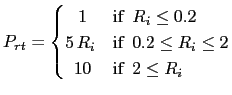
Options are defined through the namzdf namelist variables. When key_ zdfcst is defined, the momentum and tracer vertical eddy coefficients are set to constant values over the whole ocean. This is the crudest way to define the vertical ocean physics. It is recommended that this option is only used in process studies, not in basin scale simulations. Typical values used in this case are:
These values are set through the rn_avm0 and rn_avt0 namelist parameters.
In all cases, do not use values smaller that those associated with the molecular
viscosity and diffusivity, that is
![]() for momentum,
for momentum,
![]() for temperature and
for temperature and
![]() for salinity.
for salinity.
!-----------------------------------------------------------------------
&namzdf_ric    !   richardson number dependent vertical diffusion       ("key_zdfric" )
!-----------------------------------------------------------------------
   rn_avmri    = 100.e-4   !  maximum value of the vertical viscosity
   rn_alp      =   5.      !  coefficient of the parameterization
   nn_ric      =   2       !  coefficient of the parameterization
   rn_ekmfc    =   0.7     !  Factor in the Ekman depth Equation
   rn_mldmin   =   1.0     !  minimum allowable mixed-layer depth estimate (m)
   rn_mldmax   =1000.0     !  maximum allowable mixed-layer depth estimate (m)
   rn_wtmix    =  10.0     !  vertical eddy viscosity coeff [m2/s] in the mixed-layer
   rn_wvmix    =  10.0     !  vertical eddy diffusion coeff [m2/s] in the mixed-layer
   ln_mldw     = .true.    !  Flag to use or not the mized layer depth param.
/
When key_ zdfric is defined, a local Richardson number dependent formulation
for the vertical momentum and tracer eddy coefficients is set through the namzdf_ric
namelist variables.The vertical mixing
coefficients are diagnosed from the large scale variables computed by the model.
In situ measurements have been used to link vertical turbulent activity to
large scale ocean structures. The hypothesis of a mixing mainly maintained by the
growth of Kelvin-Helmholtz like instabilities leads to a dependency between the
vertical eddy coefficients and the local Richardson number (![]() the
ratio of stratification to vertical shear). Following Pacanowski and Philander [1981], the following
formulation has been implemented:
the
ratio of stratification to vertical shear). Following Pacanowski and Philander [1981], the following
formulation has been implemented:
A simple mixing-layer model to transfer and dissipate the atmospheric forcings (wind-stress and buoyancy fluxes) can be activated setting the ln_mldw =.true. in the namelist.
In this case, the local depth of turbulent wind-mixing or "Ekman depth"
![]() is evaluated and the vertical eddy coefficients prescribed within this layer.
is evaluated and the vertical eddy coefficients prescribed within this layer.
This depth is assumed proportional to the "depth of frictional influence" that is limited by rotation:
 |
(10.2) |
In this similarity height relationship, the turbulent friction velocity:
 |
(10.3) |
is computed from the wind stress vector ![]() and the reference density
and the reference density ![]() .
The final
.
The final ![]() is further constrained by the adjustable bounds rn_mldmin and rn_mldmax.
Once
is further constrained by the adjustable bounds rn_mldmin and rn_mldmax.
Once ![]() is computed, the vertical eddy coefficients within
is computed, the vertical eddy coefficients within ![]() are set to
the empirical values rn_wtmix and rn_wvmix [Lermusiaux, 2001].
are set to
the empirical values rn_wtmix and rn_wvmix [Lermusiaux, 2001].
!-----------------------------------------------------------------------
&namzdf_tke    !   turbulent eddy kinetic dependent vertical diffusion  ("key_zdftke")
!-----------------------------------------------------------------------
   rn_ediff    =   0.1     !  coef. for vertical eddy coef. (avt=rn_ediff*mxl*sqrt(e) )
   rn_ediss    =   0.7     !  coef. of the Kolmogoroff dissipation
   rn_ebb      =  67.83    !  coef. of the surface input of tke (=67.83 suggested when ln_mxl0=T)
   rn_emin     =   1.e-6   !  minimum value of tke [m2/s2]
   rn_emin0    =   1.e-4   !  surface minimum value of tke [m2/s2]
   rn_bshear   =   1.e-20  ! background shear (>0) currently a numerical threshold (do not change it)
   nn_mxl      =   2       !  mixing length: = 0 bounded by the distance to surface and bottom
                           !                 = 1 bounded by the local vertical scale factor
                           !                 = 2 first vertical derivative of mixing length bounded by 1
                           !                 = 3 as =2 with distinct disspipative an mixing length scale
   nn_pdl      =   1       !  Prandtl number function of richarson number (=1, avt=pdl(Ri)*avm) or not (=0, avt=avm)
   ln_mxl0     = .true.    !  surface mixing length scale = F(wind stress) (T) or not (F)
   rn_mxl0     =   0.04    !  surface  buoyancy lenght scale minimum value
   ln_lc       = .true.    !  Langmuir cell parameterisation (Axell 2002)
   rn_lc       =   0.15    !  coef. associated to Langmuir cells
   nn_etau     =   1       !  penetration of tke below the mixed layer (ML) due to internal & intertial waves
                           !        = 0 no penetration
                           !        = 1 add a tke source below the ML
                           !        = 2 add a tke source just at the base of the ML
                           !        = 3 as = 1 applied on HF part of the stress    ("key_oasis3")
   rn_efr      =   0.05    !  fraction of surface tke value which penetrates below the ML (nn_etau=1 or 2)
   nn_htau     =   1       !  type of exponential decrease of tke penetration below the ML
                           !        = 0  constant 10 m length scale
                           !        = 1  0.5m at the equator to 30m poleward of 40 degrees
/
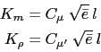
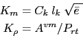
The vertical eddy viscosity and diffusivity coefficients are computed from a TKE
turbulent closure model based on a prognostic equation for ![]() , the turbulent
kinetic energy, and a closure assumption for the turbulent length scales. This
turbulent closure model has been developed by Bougeault and Lacarrere [1989] in the
atmospheric case, adapted by Gaspar et al. [1990] for the oceanic case, and
embedded in OPA, the ancestor of NEMO, by Blanke and Delecluse [1993] for equatorial Atlantic
simulations. Since then, significant modifications have been introduced by
Madec et al. [1998] in both the implementation and the formulation of the mixing
length scale. The time evolution of
, the turbulent
kinetic energy, and a closure assumption for the turbulent length scales. This
turbulent closure model has been developed by Bougeault and Lacarrere [1989] in the
atmospheric case, adapted by Gaspar et al. [1990] for the oceanic case, and
embedded in OPA, the ancestor of NEMO, by Blanke and Delecluse [1993] for equatorial Atlantic
simulations. Since then, significant modifications have been introduced by
Madec et al. [1998] in both the implementation and the formulation of the mixing
length scale. The time evolution of ![]() is the result of the production of
is the result of the production of
![]() through vertical shear, its destruction through stratification, its vertical
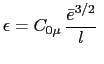
diffusion, and its dissipation of Kolmogorov [1942] type:
through vertical shear, its destruction through stratification, its vertical
diffusion, and its dissipation of Kolmogorov [1942] type:
At the sea surface, the value of ![]() is prescribed from the wind
stress field as
is prescribed from the wind
stress field as
![]() , with
, with ![]() the rn_ebb
namelist parameter. The default value of
the rn_ebb
namelist parameter. The default value of ![]() is 3.75. [Gaspar et al., 1990]),
however a much larger value can be used when taking into account the
surface wave breaking (see below Eq. (10.10)).
The bottom value of TKE is assumed to be equal to the value of the level just above.
The time integration of the
is 3.75. [Gaspar et al., 1990]),
however a much larger value can be used when taking into account the
surface wave breaking (see below Eq. (10.10)).
The bottom value of TKE is assumed to be equal to the value of the level just above.
The time integration of the ![]() equation may formally lead to negative values
because the numerical scheme does not ensure its positivity. To overcome this
problem, a cut-off in the minimum value of
equation may formally lead to negative values
because the numerical scheme does not ensure its positivity. To overcome this
problem, a cut-off in the minimum value of ![]() is used (rn_emin
namelist parameter). Following Gaspar et al. [1990], the cut-off value is set
to
is used (rn_emin
namelist parameter). Following Gaspar et al. [1990], the cut-off value is set
to
![]() . This allows the subsequent formulations
to match that of Gargett [1984] for the diffusion in the thermocline and
deep ocean :
. This allows the subsequent formulations
to match that of Gargett [1984] for the diffusion in the thermocline and
deep ocean :
![]() .
In addition, a cut-off is applied on
.
In addition, a cut-off is applied on ![]() and
and ![]() to avoid numerical
instabilities associated with too weak vertical diffusion. They must be
specified at least larger than the molecular values, and are set through
rn_avm0 and rn_avt0 (namzdf namelist, see §10.1.1).
to avoid numerical
instabilities associated with too weak vertical diffusion. They must be
specified at least larger than the molecular values, and are set through
rn_avm0 and rn_avt0 (namzdf namelist, see §10.1.1).
 .
.
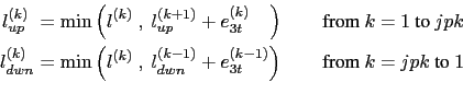
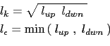
In the nn_mxl = 2 case, the dissipation and mixing length scales take the same
value:
![]() , while in the
nn_mxl = 3 case, the dissipation and mixing turbulent length scales are give
as in Gaspar et al. [1990]:
, while in the
nn_mxl = 3 case, the dissipation and mixing turbulent length scales are give
as in Gaspar et al. [1990]:
At the ocean surface, a non zero length scale is set through the rn_mxl0 namelist
parameter. Usually the surface scale is given by
![]() where
where
![]() is von Karman's constant and
is von Karman's constant and ![]() the roughness
parameter of the surface. Assuming
the roughness
parameter of the surface. Assuming ![]() m [Craig and Banner, 1994]
leads to a 0.04 m, the default value of rn_mxl0. In the ocean interior
a minimum length scale is set to recover the molecular viscosity when
m [Craig and Banner, 1994]
leads to a 0.04 m, the default value of rn_mxl0. In the ocean interior
a minimum length scale is set to recover the molecular viscosity when ![]() reach its minimum value (
reach its minimum value (
![]() ).
).
Following Craig and Banner [1994], the boundary condition on surface TKE value is :
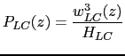
Here we introduced in the TKE turbulent closure the simple parameterization of
Langmuir circulations proposed by [Axell, 2002] for a
![]() turbulent closure.
The parameterization, tuned against large-eddy simulation, includes the whole effect
of LC in an extra source terms of TKE,
turbulent closure.
The parameterization, tuned against large-eddy simulation, includes the whole effect
of LC in an extra source terms of TKE, ![]() .
The presence of
.
The presence of ![]() in (10.4), the TKE equation, is controlled
by setting ln_lc to true in the namtke namelist.
in (10.4), the TKE equation, is controlled
by setting ln_lc to true in the namtke namelist.
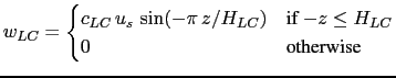
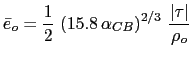
By making an analogy with the characteristic convective velocity scale
(![]() , D'Alessio et al. [1998]),
, D'Alessio et al. [1998]), ![]() is assumed to be :
is assumed to be :
 |
(10.12) |
 |
(10.13) |
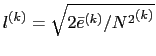
The ![]() is estimated in a similar way as the turbulent length scale of TKE equations:
is estimated in a similar way as the turbulent length scale of TKE equations:
![]() is depth to which a water parcel with kinetic energy due to Stoke drift
can reach on its own by converting its kinetic energy to potential energy, according to
is depth to which a water parcel with kinetic energy due to Stoke drift
can reach on its own by converting its kinetic energy to potential energy, according to
 |
(10.14) |
Vertical mixing parameterizations commonly used in ocean general circulation models
tend to produce mixed-layer depths that are too shallow during summer months and windy conditions.
This bias is particularly acute over the Southern Ocean.
To overcome this systematic bias, an ad hoc parameterization is introduced into the TKE scheme Rodgers et al. [2014].
The parameterization is an empirical one, ![]() not derived from theoretical considerations,
but rather is meant to account for observed processes that affect the density structure of
the ocean’s planetary boundary layer that are not explicitly captured by default in the TKE scheme
(
not derived from theoretical considerations,
but rather is meant to account for observed processes that affect the density structure of
the ocean’s planetary boundary layer that are not explicitly captured by default in the TKE scheme
(![]() near-inertial oscillations and ocean swells and waves).
near-inertial oscillations and ocean swells and waves).
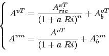
When using this parameterization (![]() when nn_etau = 1), the TKE input to the ocean (
when nn_etau = 1), the TKE input to the ocean (![]() )
imposed by the winds in the form of near-inertial oscillations, swell and waves is parameterized
by (10.10) the standard TKE surface boundary condition, plus a depth depend one given by:
)
imposed by the winds in the form of near-inertial oscillations, swell and waves is parameterized
by (10.10) the standard TKE surface boundary condition, plus a depth depend one given by:
Note that two other option existe, nn_etau = 2, or 3. They correspond to applying (10.15) only at the base of the mixed layer, or to using the high frequency part of the stress to evaluate the fraction of TKE that penetrate the ocean. Those two options are obsolescent features introduced for test purposes. They will be removed in the next release.
![\includegraphics[width=1.00\textwidth]{Fig_ZDF_TKE_time_scheme}](img982.png)
|
The production of turbulence by vertical shear (the first term of the right hand side of (10.4)) should balance the loss of kinetic energy associated with the vertical momentum diffusion (first line in (2.34)). To do so a special care have to be taken for both the time and space discretization of the TKE equation [Marsaleix et al., 2008, Burchard, 2002].
Let us first address the time stepping issue. Fig. 10.2 shows
how the two-level Leap-Frog time stepping of the momentum and tracer equations interplays
with the one-level forward time stepping of TKE equation. With this framework, the total loss
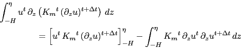
of kinetic energy (in 1D for the demonstration) due to the vertical momentum diffusion is
obtained by multiplying this quantity by ![]() and summing the result vertically:
and summing the result vertically:
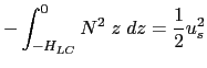
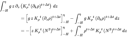
A similar consideration applies on the destruction rate of ![]() due to stratification
(second term of the right hand side of (10.4)). This term
must balance the input of potential energy resulting from vertical mixing.
The rate of change of potential energy (in 1D for the demonstration) due vertical
mixing is obtained by multiplying vertical density diffusion
tendency by
due to stratification
(second term of the right hand side of (10.4)). This term
must balance the input of potential energy resulting from vertical mixing.
The rate of change of potential energy (in 1D for the demonstration) due vertical
mixing is obtained by multiplying vertical density diffusion
tendency by ![]() and and summing the result vertically:
and and summing the result vertically:
Let us now address the space discretization issue.
The vertical eddy coefficients are defined at ![]() -point whereas the horizontal velocity
components are in the centre of the side faces of a
-point whereas the horizontal velocity
components are in the centre of the side faces of a ![]() -box in staggered C-grid
(Fig.4.1). A space averaging is thus required to obtain the shear TKE production term.
By redoing the (10.16) in the 3D case, it can be shown that the product of
eddy coefficient by the shear at
-box in staggered C-grid
(Fig.4.1). A space averaging is thus required to obtain the shear TKE production term.
By redoing the (10.16) in the 3D case, it can be shown that the product of
eddy coefficient by the shear at ![]() and
and ![]() must be performed prior to the averaging.
Furthermore, the possible time variation of
must be performed prior to the averaging.
Furthermore, the possible time variation of ![]() (key_ vvl case) have to be taken into
account.
(key_ vvl case) have to be taken into
account.
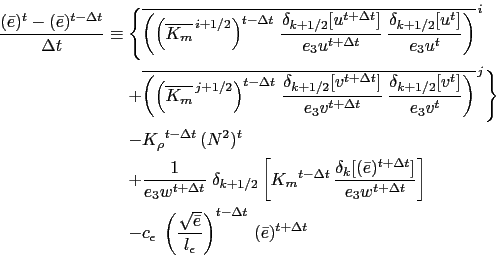
The above energetic considerations leads to the following final discrete form for the TKE equation:
!-----------------------------------------------------------------------
&namzdf_gls                !   GLS vertical diffusion                   ("key_zdfgls")
!-----------------------------------------------------------------------
   rn_emin       = 1.e-7   !  minimum value of e   [m2/s2]
   rn_epsmin     = 1.e-12  !  minimum value of eps [m2/s3]
   ln_length_lim = .true.  !  limit on the dissipation rate under stable stratification (Galperin et al., 1988)
   rn_clim_galp  = 0.267   !  galperin limit
   ln_sigpsi     = .true.  !  Activate or not Burchard 2001 mods on psi schmidt number in the wb case
   rn_crban      = 100.    !  Craig and Banner 1994 constant for wb tke flux
   rn_charn      = 70000.  !  Charnock constant for wb induced roughness length
   rn_hsro       =  0.02   !  Minimum surface roughness
   rn_frac_hs    =   1.3   !  Fraction of wave height as roughness (if nn_z0_met=2)
   nn_z0_met     =     2   !  Method for surface roughness computation (0/1/2)
   nn_bc_surf    =     1   !  surface condition (0/1=Dir/Neum)
   nn_bc_bot     =     1   !  bottom condition (0/1=Dir/Neum)
   nn_stab_func  =     2   !  stability function (0=Galp, 1= KC94, 2=CanutoA, 3=CanutoB)
   nn_clos       =     1   !  predefined closure type (0=MY82, 1=k-eps, 2=k-w, 3=Gen)
/
The Generic Length Scale (GLS) scheme is a turbulent closure scheme based on
two prognostic equations: one for the turbulent kinetic energy ![]() , and another
for the generic length scale,
, and another
for the generic length scale, ![]() [Umlauf and Burchard, 2003, Umlauf and Burchard, 2005].
This later variable is defined as :
[Umlauf and Burchard, 2003, Umlauf and Burchard, 2005].
This later variable is defined as :
![]() ,
where the triplet
,
where the triplet ![]() value given in Tab.10.1 allows to recover
a number of well-known turbulent closures (
value given in Tab.10.1 allows to recover
a number of well-known turbulent closures (![]() -
-![]() [Mellor and Yamada, 1982],
[Mellor and Yamada, 1982],
![]() -
-![]() [Rodi, 1987],
[Rodi, 1987], ![]() -
-![]() [Wilcox, 1988]
among others [Kantha and Carniel, 2005, Umlauf and Burchard, 2003]).
The GLS scheme is given by the following set of equations:
[Wilcox, 1988]
among others [Kantha and Carniel, 2005, Umlauf and Burchard, 2003]).
The GLS scheme is given by the following set of equations:
In the Mellor-Yamada model, the negativity of ![]() allows to use a wall function to force
the convergence of the mixing length towards
allows to use a wall function to force
the convergence of the mixing length towards ![]() (
(![]() : Kappa and
: Kappa and ![]() : rugosity length)
value near physical boundaries (logarithmic boundary layer law).
: rugosity length)
value near physical boundaries (logarithmic boundary layer law). ![]() and
and ![]() are calculated from stability function proposed by Galperin et al. [1988], or by Kantha and Clayson [1994]
or one of the two functions suggested by Canuto et al. [2001] (nn_stab_func = 0, 1, 2 or 3, resp.).
The value of
are calculated from stability function proposed by Galperin et al. [1988], or by Kantha and Clayson [1994]
or one of the two functions suggested by Canuto et al. [2001] (nn_stab_func = 0, 1, 2 or 3, resp.).
The value of ![]() depends of the choice of the stability function.
depends of the choice of the stability function.
The surface and bottom boundary condition on both ![]() and
and ![]() can be calculated
thanks to Dirichlet or Neumann condition through nn_tkebc_surf and nn_tkebc_bot, resp.
As for TKE closure , the wave effect on the mixing is considered when ln_crban = true
[Mellor and Blumberg, 2004, Craig and Banner, 1994]. The rn_crban namelist parameter
is
can be calculated
thanks to Dirichlet or Neumann condition through nn_tkebc_surf and nn_tkebc_bot, resp.
As for TKE closure , the wave effect on the mixing is considered when ln_crban = true
[Mellor and Blumberg, 2004, Craig and Banner, 1994]. The rn_crban namelist parameter
is
![]() in (10.10) and rn_charn provides the value of
in (10.10) and rn_charn provides the value of ![]() in (10.11).
in (10.11).
The ![]() equation is known to fail in stably stratified flows, and for this reason
almost all authors apply a clipping of the length scale as an ad hoc remedy.
With this clipping, the maximum permissible length scale is determined by
equation is known to fail in stably stratified flows, and for this reason
almost all authors apply a clipping of the length scale as an ad hoc remedy.
With this clipping, the maximum permissible length scale is determined by
![]() . A value of
. A value of
![]() is often used
[Galperin et al., 1988]. Umlauf and Burchard [2005] show that the value of
the clipping factor is of crucial importance for the entrainment depth predicted in
stably stratified situations, and that its value has to be chosen in accordance
with the algebraic model for the turbulent fluxes. The clipping is only activated
if ln_length_lim=true, and the
is often used
[Galperin et al., 1988]. Umlauf and Burchard [2005] show that the value of
the clipping factor is of crucial importance for the entrainment depth predicted in
stably stratified situations, and that its value has to be chosen in accordance
with the algebraic model for the turbulent fluxes. The clipping is only activated
if ln_length_lim=true, and the ![]() is set to the rn_clim_galp value.
is set to the rn_clim_galp value.
The time and space discretization of the GLS equations follows the same energetic consideration as for the TKE case described in §10.1.4 [Burchard, 2002]. Examples of performance of the 4 turbulent closure scheme can be found in Warner et al. [2005].
!------------------------------------------------------------------------
&namzdf_kpp    !   K-Profile Parameterization dependent vertical mixing  ("key_zdfkpp", and optionally:
!------------------------------------------------------------------------ "key_kppcustom" or "key_kpplktb")
   ln_kpprimix = .true.    !  shear instability mixing
   rn_difmiw   =  1.0e-04  !  constant internal wave viscosity [m2/s]
   rn_difsiw   =  0.1e-04  !  constant internal wave diffusivity [m2/s]
   rn_riinfty  =  0.8      !  local Richardson Number limit for shear instability
   rn_difri    =  0.0050   !  maximum shear mixing at Rig = 0    [m2/s]
   rn_bvsqcon  = -0.01e-07 !  Brunt-Vaisala squared for maximum convection [1/s2]
   rn_difcon   =  1.       !  maximum mixing in interior convection [m2/s]
   nn_avb      =  0        !  horizontal averaged (=1) or not (=0) on avt and amv
   nn_ave      =  1        !  constant (=0) or profile (=1) background on avt
/
The KKP scheme has been implemented by J. Chanut ... Options are defined through the namzdf_kpp namelist variables.
Note that KPP is an obsolescent feature of the NEMO system. It will be removed in the next release (v3.7 and followings).
Gurvan Madec and the NEMO Team
NEMO European Consortium2017-02-17
![$\displaystyle \frac{\partial \bar{e}}{\partial t} = \frac{K_m}{{e_3}^2 }\;\left...
...\bar{e}}{\partial k}} \right] - c_\epsilon \;\frac{\bar {e}^{3/2}}{l_\epsilon }$](img922.png)
 with
with ![\includegraphics[width=1.00\textwidth]{Fig_mixing_length}](img943.png)

![$\displaystyle \frac{\partial \bar{e}}{\partial t} = \frac{K_m}{\sigma_e e_3 }\;...
... \left[ \frac{K_m}{e_3} \frac{\partial \bar{e}}{\partial k} \right] - \epsilon$](img1000.png)
![\begin{displaymath}\begin{split}\frac{\partial \psi}{\partial t} =& \frac{\psi}{...
...e_3 } \;\frac{\partial \psi}{\partial k}} \right]\; \end{split}\end{displaymath}](img1001.png)