Next: Domain: Horizontal Grid (mesh) Up: Space Domain (DOM) Previous: Space Domain (DOM) Contents Index
![\includegraphics[width=0.90\textwidth]{Fig_cell}](img315.png)
|
The numerical techniques used to solve the Primitive Equations in this model are
based on the traditional, centred second-order finite difference approximation.
Special attention has been given to the homogeneity of the solution in the three
space directions. The arrangement of variables is the same in all directions.
It consists of cells centred on scalar points (![]() ,
, ![]() ,
, ![]() ,
, ![]() ) with vector
points
) with vector
points ![]() defined in the centre of each face of the cells (Fig. 4.1).
This is the generalisation to three dimensions of the well-known “C” grid in
Arakawa's classification [Mesinger and Arakawa, 1976]. The relative and
planetary vorticity,
defined in the centre of each face of the cells (Fig. 4.1).
This is the generalisation to three dimensions of the well-known “C” grid in
Arakawa's classification [Mesinger and Arakawa, 1976]. The relative and
planetary vorticity, ![]() and
and ![]() , are defined in the centre of each vertical edge
and the barotropic stream function
, are defined in the centre of each vertical edge
and the barotropic stream function ![]() is defined at horizontal points overlying
the
is defined at horizontal points overlying
the ![]() and
and ![]() -points.
-points.
The ocean mesh (![]() the position of all the scalar and vector points) is defined
by the transformation that gives (
the position of all the scalar and vector points) is defined
by the transformation that gives (![]() ,
,![]() ,
,![]() ) as a function of
) as a function of ![]() .
The grid-points are located at integer or integer and a half value of
.
The grid-points are located at integer or integer and a half value of ![]() as
indicated on Table 4.1. In all the following, subscripts
as
indicated on Table 4.1. In all the following, subscripts ![]() ,
,  ,
, ![]() ,
,
![]() ,
, ![]() ,
, ![]() or
or ![]() indicate the position of the grid-point where the scale
factors are defined. Each scale factor is defined as the local analytical value
provided by (2.6). As a result, the mesh on which partial
derivatives
indicate the position of the grid-point where the scale
factors are defined. Each scale factor is defined as the local analytical value
provided by (2.6). As a result, the mesh on which partial
derivatives
![]() , and
, and
![]() are evaluated is a uniform mesh with a grid size of unity.
Discrete partial derivatives are formulated by the traditional, centred second order
finite difference approximation while the scale factors are chosen equal to their
local analytical value. An important point here is that the partial derivative of the
scale factors must be evaluated by centred finite difference approximation, not
from their analytical expression. This preserves the symmetry of the discrete set
of equations and therefore satisfies many of the continuous properties (see
Appendix C). A similar, related remark can be made about the domain
size: when needed, an area, volume, or the total ocean depth must be evaluated
as the sum of the relevant scale factors (see (4.8)) in the next section).
are evaluated is a uniform mesh with a grid size of unity.
Discrete partial derivatives are formulated by the traditional, centred second order
finite difference approximation while the scale factors are chosen equal to their
local analytical value. An important point here is that the partial derivative of the
scale factors must be evaluated by centred finite difference approximation, not
from their analytical expression. This preserves the symmetry of the discrete set
of equations and therefore satisfies many of the continuous properties (see
Appendix C). A similar, related remark can be made about the domain
size: when needed, an area, volume, or the total ocean depth must be evaluated
as the sum of the relevant scale factors (see (4.8)) in the next section).
|
Given the values of a variable ![]() at adjacent points, the differencing and
averaging operators at the midpoint between them are:
at adjacent points, the differencing and
averaging operators at the midpoint between them are:
Similar operators are defined with respect to ![]() ,
, ![]() ,
, ![]() ,
, ![]() , and
, and
![]() . Following (2.7a) and (2.7d), the gradient of a
variable
. Following (2.7a) and (2.7d), the gradient of a
variable ![]() defined at a
defined at a ![]() -point has its three components defined at
-point has its three components defined at ![]() -, -
and
-, -
and ![]() -points while its Laplacien is defined at
-points while its Laplacien is defined at ![]() -point. These operators have
the following discrete forms in the curvilinear
-point. These operators have
the following discrete forms in the curvilinear ![]() -coordinate system:
-coordinate system:
Following (2.7c) and (2.7b), a vector
![]() defined at vector points
defined at vector points ![]() has its three curl components defined at
has its three curl components defined at ![]() -,
-, ![]() ,
and
,
and ![]() -points, and its divergence defined at
-points, and its divergence defined at ![]() -points:
-points:
In the special case of a pure ![]() -coordinate system, (4.3) and
(4.7) can be simplified. In this case, the vertical scale factor
becomes a function of the single variable
-coordinate system, (4.3) and
(4.7) can be simplified. In this case, the vertical scale factor
becomes a function of the single variable ![]() and thus does not depend on the
horizontal location of a grid point. For example (4.7) reduces to:
and thus does not depend on the
horizontal location of a grid point. For example (4.7) reduces to:
![$\displaystyle \nabla \cdot \rm {\bf A}=\frac{1}{e_{1t} e_{2t}} \left( \delta_i...
...left[e_{1v} a_2 \right] \right) +\frac{1}{e_{3t}} \delta_k \left[ a_3 \right]$](img341.png) |
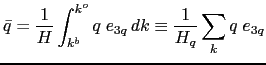
The vertical average over the whole water column denoted by an overbar becomes
for a quantity ![]() which is a masked field (i.e. equal to zero inside solid area):
which is a masked field (i.e. equal to zero inside solid area):
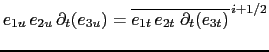
In continuous form, the following properties are satisfied:
It is straightforward to demonstrate that these properties are verified locally in
discrete form as soon as the scalar ![]() is taken at
is taken at ![]() -points and the vector
A has its components defined at vector points
-points and the vector
A has its components defined at vector points ![]() .
.
Let ![]() and
and ![]() be two fields defined on the mesh, with value zero inside
continental area. Using integration by parts it can be shown that the differencing
operators (
be two fields defined on the mesh, with value zero inside
continental area. Using integration by parts it can be shown that the differencing
operators (![]() ,
, ![]() and
and ![]() ) are skew-symmetric linear operators,
and further that the averaging operators
) are skew-symmetric linear operators,
and further that the averaging operators
![]() ,
,
![]() and
and
![]() ) are symmetric linear
operators,
) are symmetric linear
operators, ![]()
In other words, the adjoint of the differencing and averaging operators are
![]() and
and
![]() , respectively.
These two properties will be used extensively in the Appendix C to
demonstrate integral conservative properties of the discrete formulation chosen.
, respectively.
These two properties will be used extensively in the Appendix C to
demonstrate integral conservative properties of the discrete formulation chosen.
![\includegraphics[width=0.90\textwidth]{Fig_index_hor}](img360.png)
|
The array representation used in the FORTRAN code requires an integer
indexing while the analytical definition of the mesh (see §4.1.1) is
associated with the use of integer values for ![]() -points and both integer and
integer and a half values for all the other points. Therefore a specific integer
indexing must be defined for points other than
-points and both integer and
integer and a half values for all the other points. Therefore a specific integer
indexing must be defined for points other than ![]() -points (
-points (![]() velocity and
vorticity grid-points). Furthermore, the direction of the vertical indexing has
been changed so that the surface level is at
velocity and
vorticity grid-points). Furthermore, the direction of the vertical indexing has
been changed so that the surface level is at ![]() .
.
The indexing in the horizontal plane has been chosen as shown in Fig.4.2.
For an increasing ![]() index (
index (![]() index), the
index), the ![]() -point and the eastward
-point and the eastward ![]() -point
(northward -point) have the same index (see the dashed area in Fig.4.2).
A
-point
(northward -point) have the same index (see the dashed area in Fig.4.2).
A ![]() -point and its nearest northeast
-point and its nearest northeast ![]() -point have the same
-point have the same ![]() -and
-and ![]() -indices.
-indices.
In the vertical, the chosen indexing requires special attention since the
![]() -axis is re-orientated downward in the FORTRAN code compared
to the indexing used in the semi-discrete equations and given in §4.1.1.
The sea surface corresponds to the
-axis is re-orientated downward in the FORTRAN code compared
to the indexing used in the semi-discrete equations and given in §4.1.1.
The sea surface corresponds to the ![]() -level
-level ![]() which is the same index
as
which is the same index
as ![]() -level just below (Fig.4.3). The last
-level just below (Fig.4.3). The last ![]() -level (
-level (![]() )
either corresponds to the ocean floor or is inside the bathymetry while the last
)
either corresponds to the ocean floor or is inside the bathymetry while the last
![]() -level is always inside the bathymetry (Fig.4.3). Note that
for an increasing
-level is always inside the bathymetry (Fig.4.3). Note that
for an increasing ![]() index, a
index, a ![]() -point and the
-point and the ![]() -point just below have the
same
-point just below have the
same ![]() index, in opposition to what is done in the horizontal plane where
it is the
index, in opposition to what is done in the horizontal plane where
it is the ![]() -point and the nearest velocity points in the direction of the horizontal
axis that have the same
-point and the nearest velocity points in the direction of the horizontal
axis that have the same ![]() or
or ![]() index (compare the dashed area in
Fig.4.2 and 4.3). Since the scale factors are
chosen to be strictly positive, a minus sign appears in the FORTRAN
code before all the vertical derivatives of the discrete equations given in
this documentation.
index (compare the dashed area in
Fig.4.2 and 4.3). Since the scale factors are
chosen to be strictly positive, a minus sign appears in the FORTRAN
code before all the vertical derivatives of the discrete equations given in
this documentation.
![\includegraphics[width=.90\textwidth]{Fig_index_vert}](img362.png)
|
The total size of the computational domain is set by the parameters jpiglo,
jpjglo and jpkdta in the ![]() ,
, ![]() and
and ![]() directions respectively. They are
given as namelist variables in the namcfg namelist.
directions respectively. They are
given as namelist variables in the namcfg namelist.
Note that are other namelist variables in the namcfg namelist that refer to
the domain size.
The two variables jpidta and jpjdta may be larger than jpiglo, jpjglo
when the user wants to use only a sub-region of a given configuration. This is
the "zoom" capability described in §15.3. In most applications of
the model,
![]() ,
,
![]() , and
, and
![]() . Parameters
. Parameters
![]() and
and ![]() refer to the size of each processor subdomain when the code is
run in parallel using domain decomposition (key_ mpp_mpi defined, see
§8.3).
refer to the size of each processor subdomain when the code is
run in parallel using domain decomposition (key_ mpp_mpi defined, see
§8.3).
![]()
Gurvan Madec and the NEMO Team
NEMO European Consortium2017-02-17
![\begin{subequations}\begin{align}\delta _i [q] &= q(i+1/2) - q(i-1/2) \ov...
... &= \left\{ q(i+1/2) + q(i-1/2) \right\} \; / \; 2 \end{align}\end{subequations}](img328.png)
![$\displaystyle \nabla q\equiv \frac{1}{e_{1u} } \delta _{i+1/2 } [q] \; \mathbf...
...+1/2 } [q] \; \mathbf{j} + \frac{1}{e_{3w}} \delta _{k+1/2} [q] \; \mathbf{k}$](img329.png)
![\begin{multline}
\Delta q\equiv \frac{1}{e_{1t} e_{2t} e_{3t} }
\;\left( \del...
...}} \delta_k \left[ \frac{1}{e_{3w} } \;\delta_{k+1/2} [q] \right]
\end{multline}](img330.png)
![$\displaystyle \frac{1}{e_{2v} e_{3vw} } \left( \delta_{j +1/2} \left[e_{3w} a_3 \right] -\delta_{k+1/2} \left[e_{2v} a_2 \right] \right)$](img333.png)
![$\displaystyle \frac{1}{e_{2u} e_{3uw}} \left( \delta_{k+1/2} \left[e_{1u} a_1 \right] -\delta_{i +1/2} \left[e_{3w} a_3 \right] \right)$](img336.png)
![$\displaystyle \frac{1}{e_{1f} e_{2f} } \left( \delta_{i +1/2} \left[e_{2v} a_2 \right] -\delta_{j +1/2} \left[e_{1u} a_1 \right] \right)$](img338.png)
![$\displaystyle \nabla \cdot \rm {\bf A}=\frac{1}{e_{1t} e_{2t} e_{3t}}\left( \...
...e_{1v} e_{3v} a_2 \right] \right)+\frac{1}{e_{3t} }\delta_k \left[a_3 \right]$](img340.png)
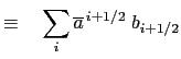
![$\displaystyle \sum\limits_i { a_i \;\delta _i \left[ b \right]}$](img354.png)
![$\displaystyle \equiv -\sum\limits_i {\delta _{i+1/2} \left[ a \right]\;b_{i+1/2} }$](img355.png)