Next: Curvilinear generalised vertical coordinate Up: Model basics Previous: The Horizontal Pressure Gradient Contents Index
In many ocean circulation problems, the flow field has regions of enhanced dynamics
(![]() surface layers, western boundary currents, equatorial currents, or ocean fronts).
The representation of such dynamical processes can be improved by specifically increasing
the model resolution in these regions. As well, it may be convenient to use a lateral
boundary-following coordinate system to better represent coastal dynamics. Moreover,
the common geographical coordinate system has a singular point at the North Pole that
cannot be easily treated in a global model without filtering. A solution consists of introducing
an appropriate coordinate transformation that shifts the singular point onto land
[Murray, 1996, Madec and Imbard, 1996]. As a consequence, it is important to solve the primitive
equations in various curvilinear coordinate systems. An efficient way of introducing an
appropriate coordinate transform can be found when using a tensorial formalism.
This formalism is suited to any multidimensional curvilinear coordinate system. Ocean
modellers mainly use three-dimensional orthogonal grids on the sphere (spherical earth
approximation), with preservation of the local vertical. Here we give the simplified equations
for this particular case. The general case is detailed by Eiseman and Stone [1980] in their survey
of the conservation laws of fluid dynamics.
surface layers, western boundary currents, equatorial currents, or ocean fronts).
The representation of such dynamical processes can be improved by specifically increasing
the model resolution in these regions. As well, it may be convenient to use a lateral
boundary-following coordinate system to better represent coastal dynamics. Moreover,
the common geographical coordinate system has a singular point at the North Pole that
cannot be easily treated in a global model without filtering. A solution consists of introducing
an appropriate coordinate transformation that shifts the singular point onto land
[Murray, 1996, Madec and Imbard, 1996]. As a consequence, it is important to solve the primitive
equations in various curvilinear coordinate systems. An efficient way of introducing an
appropriate coordinate transform can be found when using a tensorial formalism.
This formalism is suited to any multidimensional curvilinear coordinate system. Ocean
modellers mainly use three-dimensional orthogonal grids on the sphere (spherical earth
approximation), with preservation of the local vertical. Here we give the simplified equations
for this particular case. The general case is detailed by Eiseman and Stone [1980] in their survey
of the conservation laws of fluid dynamics.
Let (i,j,k) be a set of orthogonal curvilinear coordinates on the sphere
associated with the positively oriented orthogonal set of unit vectors (i,j,k)
linked to the earth such that k is the local upward vector and (i,j) are
two vectors orthogonal to k, ![]() along geopotential surfaces (Fig.2.2).
Let
along geopotential surfaces (Fig.2.2).
Let
![]() be the geographical coordinate system in which a position is defined
by the latitude
be the geographical coordinate system in which a position is defined
by the latitude
![]() , the longitude
, the longitude
![]() and the distance from the centre of
the earth
and the distance from the centre of
the earth ![]() where
where ![]() is the earth's radius and
is the earth's radius and ![]() the altitude above a reference sea
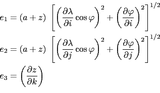
level (Fig.2.2). The local deformation of the curvilinear coordinate system is
given by
the altitude above a reference sea
level (Fig.2.2). The local deformation of the curvilinear coordinate system is
given by ![]() ,
, ![]() and
and ![]() , the three scale factors:
, the three scale factors:
Since the ocean depth is far smaller than the earth's radius, ![]() , can be replaced by
, can be replaced by
![]() in (2.6) (thin-shell approximation). The resulting horizontal scale
factors
in (2.6) (thin-shell approximation). The resulting horizontal scale
factors ![]() ,
, ![]() are independent of
are independent of ![]() while the vertical scale factor is a single
function of
while the vertical scale factor is a single
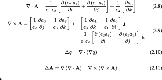
function of ![]() as k is parallel to z. The scalar and vector operators that
appear in the primitive equations (Eqs. (2.1a) to (2.1f)) can
be written in the tensorial form, invariant in any orthogonal horizontal curvilinear coordinate
system transformation:
as k is parallel to z. The scalar and vector operators that
appear in the primitive equations (Eqs. (2.1a) to (2.1f)) can
be written in the tensorial form, invariant in any orthogonal horizontal curvilinear coordinate
system transformation:
In order to express the Primitive Equations in tensorial formalism, it is necessary to compute
the horizontal component of the non-linear and viscous terms of the equation using
(2.7a)) to (2.7e).
Let us set
![]() , the velocity in the
, the velocity in the ![]() coordinate
system and define the relative vorticity
coordinate
system and define the relative vorticity ![]() and the divergence of the horizontal velocity
field
and the divergence of the horizontal velocity
field ![]() , by:
, by:
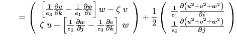
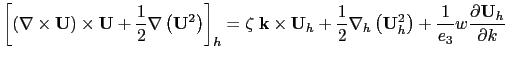
Using the fact that the horizontal scale factors ![]() and
and ![]() are independent of
are independent of ![]() and that
and that ![]() is a function of the single variable
is a function of the single variable ![]() , the nonlinear term of
(2.1a) can be transformed as follows:
, the nonlinear term of
(2.1a) can be transformed as follows:
![$\displaystyle \left[ {\left( { \nabla \times {\rm {\bf U}} } \right) \times {\rm {\bf U}} +\frac{1}{2} \nabla \left( {{\rm {\bf U}}^2} \right)} \right]_h$](img158.png) |
 |
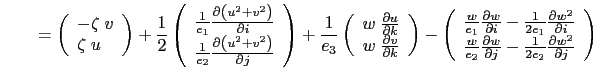 |
The last term of the right hand side is obviously zero, and thus the nonlinear term of
(2.1a) is written in the ![]() coordinate system:
coordinate system:
This is the so-called vector invariant form of the momentum advection term.
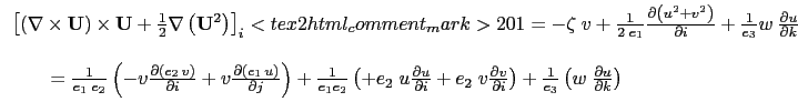
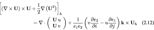
For some purposes, it can be advantageous to write this term in the so-called flux form,
![]() to write it as the divergence of fluxes. For example, the first component of
(2.10) (the
to write it as the divergence of fluxes. For example, the first component of
(2.10) (the ![]() -component) is transformed as follows:
-component) is transformed as follows:
 |
 |
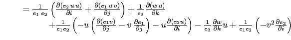 |
 |
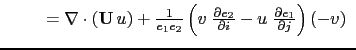 |
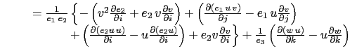
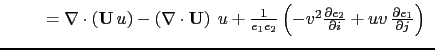
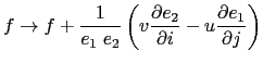
The flux form of the momentum advection term is therefore given by:
The flux form has two terms, the first one is expressed as the divergence of momentum fluxes (hence the flux form name given to this formulation) and the second one is due to the curvilinear nature of the coordinate system used. The latter is called the metric term and can be viewed as a modification of the Coriolis parameter:
Note that in the case of geographical coordinate, ![]() when
when
![]() and
and
![]() , we recover the commonly used modification of
the Coriolis parameter
, we recover the commonly used modification of
the Coriolis parameter
![]() .
.
![]()
To sum up, the curvilinear ![]() -coordinate equations solved by the ocean model can be
written in the following tensorial formalism:
-coordinate equations solved by the ocean model can be
written in the following tensorial formalism:
![]() Vector invariant form of the momentum equations :
Vector invariant form of the momentum equations :
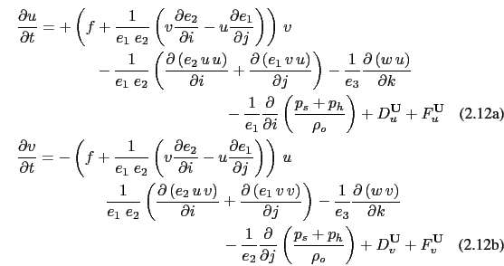
![]() flux form of the momentum equations :
flux form of the momentum equations :
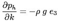
The vertical velocity and the hydrostatic pressure are diagnosed from the following equations:
![]() tracer equations :
tracer equations :
The expression of D![]() ,
, ![]() and
and ![]() depends on the subgrid scale
parameterisation used. It will be defined in §2.5.1. The nature and formulation of
depends on the subgrid scale
parameterisation used. It will be defined in §2.5.1. The nature and formulation of
![]() ,
, ![]() and
and ![]() , the surface forcing terms, are discussed
in Chapter 7.
, the surface forcing terms, are discussed
in Chapter 7.
![]()
Gurvan Madec and the NEMO Team
NEMO European Consortium2017-02-17
![\includegraphics[width=0.60\textwidth]{Fig_I_earth_referential}](img149.png)
![$\displaystyle \zeta =\frac{1}{e_1 e_2 }\left[ {\frac{\partial \left( {e_2 v} \right)}{\partial i}-\frac{\partial \left( {e_1 u} \right)}{\partial j}} \right]$](img156.png)
![$\displaystyle \chi =\frac{1}{e_1 e_2 }\left[ {\frac{\partial \left( {e_2 u} \right)}{\partial i}+\frac{\partial \left( {e_1 v} \right)}{\partial j}} \right]$](img157.png)


![$\displaystyle \frac{\partial T}{\partial t} = -\frac{1}{e_1 e_2 }\left[ { \frac...
...t] -\frac{1}{e_3 }\frac{\partial \left( {T w} \right)}{\partial k} + D^T + F^T$](img178.png)
![$\displaystyle \frac{\partial S}{\partial t} = -\frac{1}{e_1 e_2 }\left[ {\frac{...
...t] -\frac{1}{e_3 }\frac{\partial \left( {S w} \right)}{\partial k} + D^S + F^S$](img179.png)