Next: Subgrid Scale Physics Up: Model basics Previous: Curvilinear z-coordinate System Contents Index
The ocean domain presents a huge diversity of situation in the vertical. First the ocean surface is a time dependent surface (moving surface). Second the ocean floor depends on the geographical position, varying from more than 6,000 meters in abyssal trenches to zero at the coast. Last but not least, the ocean stratification exerts a strong barrier to vertical motions and mixing.
Therefore, in order to represent the ocean with respect to the first point a space and time dependent vertical coordinate that follows the variation of the sea surface height ![]() an
an ![]() *-coordinate; for the second point, a space variation to fit the change of bottom topography
*-coordinate; for the second point, a space variation to fit the change of bottom topography ![]() a terrain-following or
a terrain-following or ![]() -coordinate; and for the third point, one will be tempted to use a space and time dependent coordinate that follows the isopycnal surfaces,
-coordinate; and for the third point, one will be tempted to use a space and time dependent coordinate that follows the isopycnal surfaces, ![]() an isopycnic coordinate.
an isopycnic coordinate.
In order to satisfy two or more constrains one can even be tempted to mixed these coordinate systems, as in HYCOM (mixture of ![]() -coordinate at the surface, isopycnic coordinate in the ocean interior and
-coordinate at the surface, isopycnic coordinate in the ocean interior and ![]() at the ocean bottom) [Chassignet et al., 2003] or OPA (mixture of
at the ocean bottom) [Chassignet et al., 2003] or OPA (mixture of ![]() -coordinate in vicinity the surface and steep topography areas and
-coordinate in vicinity the surface and steep topography areas and ![]() -coordinate elsewhere) [Madec et al., 1996] among others.
-coordinate elsewhere) [Madec et al., 1996] among others.
In fact one is totally free to choose any space and time vertical coordinate by introducing an arbitrary vertical coordinate :
the generalized vertical coordinates used in ocean modelling are not orthogonal, which contrasts with many other applications in mathematical physics. Hence, it is useful to keep in mind the following properties that may seem odd on initial encounter.
The horizontal velocity in ocean models measures motions in the horizontal plane, perpendicular to the local gravitational field. That is, horizontal velocity is mathematically the same regardless the vertical coordinate, be it geopotential, isopycnal, pressure, or terrain following. The key motivation for maintaining the same horizontal velocity component is that the hydrostatic and geostrophic balances are dominant in the large-scale ocean. Use of an alternative quasi-horizontal velocity, for example one oriented parallel to the generalized surface, would lead to unacceptable numerical errors. Correspondingly, the vertical direction is anti-parallel to the gravitational force in all of the coordinate systems. We do not choose the alternative of a quasi-vertical direction oriented normal to the surface of a constant generalized vertical coordinate.
It is the method used to measure transport across the generalized vertical coordinate surfaces which differs between the vertical coordinate choices. That is, computation of the dia-surface velocity component represents the fundamental distinction between the various coordinates. In some models, such as geopotential, pressure, and terrain following, this transport is typically diagnosed from volume or mass conservation. In other models, such as isopycnal layered models, this transport is prescribed based on assumptions about the physical processes producing a flux across the layer interfaces.
In this section we first establish the PE in the generalised vertical ![]() -coordinate,
then we discuss the particular cases available in NEMO, namely
-coordinate,
then we discuss the particular cases available in NEMO, namely ![]() ,
, ![]() *,
*, ![]() , and
, and ![]() .
.
Starting from the set of equations established in §2.3 for the special case ![]() and thus
and thus ![]() , we introduce an arbitrary vertical coordinate
, we introduce an arbitrary vertical coordinate
![]() , which includes
, which includes
![]() -, z*- and
-, z*- and ![]() coordinates as special cases (
coordinates as special cases (![]() ,
,
![]() , and
, and
![]() or
or
![]() , resp.). A formal derivation of the transformed
equations is given in Appendix A. Let us define the vertical scale factor by
, resp.). A formal derivation of the transformed
equations is given in Appendix A. Let us define the vertical scale factor by
![]() (
(![]() is now a function of
is now a function of ![]() ), and the slopes in the
(i,j) directions between
), and the slopes in the
(i,j) directions between ![]() and
and ![]() surfaces by :
surfaces by :
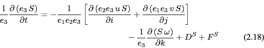
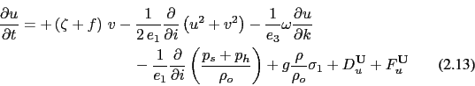
The equations solved by the ocean model (2.1) in ![]() coordinate can be written as follows (see Appendix A.3):
coordinate can be written as follows (see Appendix A.3):
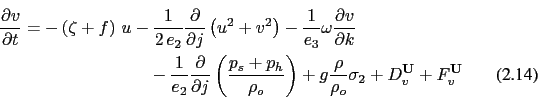
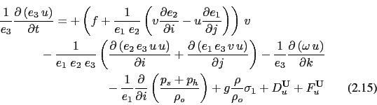
![]() Vector invariant form of the momentum equation :
Vector invariant form of the momentum equation :
![]() Vector invariant form of the momentum equation :
Vector invariant form of the momentum equation :
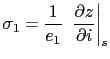
where the relative vorticity, ![]() , the surface pressure gradient, and the hydrostatic
pressure have the same expressions as in
, the surface pressure gradient, and the hydrostatic
pressure have the same expressions as in ![]() -coordinates although they do not represent
exactly the same quantities.
-coordinates although they do not represent
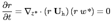
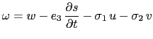
exactly the same quantities. ![]() is provided by the continuity equation
(see Appendix A):
is provided by the continuity equation
(see Appendix A):
![]() tracer equations:
tracer equations:
The equation of state has the same expression as in ![]() -coordinate, and similar expressions
are used for mixing and forcing terms.
-coordinate, and similar expressions
are used for mixing and forcing terms.
![\includegraphics[width=1.0\textwidth]{Fig_z_zstar}](img210.png)
|
In that case, the free surface equation is nonlinear, and the variations of volume are fully taken into account. These coordinates systems is presented in a report [Levier et al., 2007] available on the NEMO web site.
The z* coordinate approach is an unapproximated, non-linear free surface implementation
which allows one to deal with large amplitude free-surface
variations relative to the vertical resolution [Adcroft and Campin, 2004]. In
the z* formulation, the variation of the column thickness due to sea-surface
undulations is not concentrated in the surface level, as in the ![]() -coordinate formulation,
but is equally distributed over the full water column. Thus vertical
levels naturally follow sea-surface variations, with a linear attenuation with
depth, as illustrated by figure fig.1c . Note that with a flat bottom, such as in
fig.1c, the bottom-following
-coordinate formulation,
but is equally distributed over the full water column. Thus vertical
levels naturally follow sea-surface variations, with a linear attenuation with
depth, as illustrated by figure fig.1c . Note that with a flat bottom, such as in
fig.1c, the bottom-following ![]() coordinate and z* are equivalent.
The definition and modified oceanic equations for the rescaled vertical coordinate
z*, including the treatment of fresh-water flux at the surface, are
detailed in Adcroft and Campin (2004). The major points are summarized
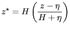
here. The position ( z*) and vertical discretization (z*) are expressed as:
coordinate and z* are equivalent.
The definition and modified oceanic equations for the rescaled vertical coordinate
z*, including the treatment of fresh-water flux at the surface, are
detailed in Adcroft and Campin (2004). The major points are summarized
here. The position ( z*) and vertical discretization (z*) are expressed as:
 |
To overcome problems with vanishing surface and/or bottom cells, we consider the zstar coordinate
This coordinate is closely related to the "eta" coordinate used in many atmospheric models (see Black (1994) for a review of eta coordinate atmospheric models). It was originally used in ocean models by Stacey et al. (1995) for studies of tides next to shelves, and it has been recently promoted by Adcroft and Campin (2004) for global climate modelling.
The surfaces of constant ![]() are quasi-horizontal. Indeed, the
are quasi-horizontal. Indeed, the ![]() coordinate reduces to
coordinate reduces to ![]() when
when ![]() is zero. In general, when noting the large differences between
undulations of the bottom topography versus undulations in the surface height, it
is clear that surfaces constant
is zero. In general, when noting the large differences between
undulations of the bottom topography versus undulations in the surface height, it
is clear that surfaces constant ![]() are very similar to the depth surfaces. These properties greatly reduce difficulties of computing the horizontal pressure gradient relative to terrain following sigma models discussed in §2.4.3.
Additionally, since
are very similar to the depth surfaces. These properties greatly reduce difficulties of computing the horizontal pressure gradient relative to terrain following sigma models discussed in §2.4.3.
Additionally, since ![]() when
when ![]() , no flow is spontaneously generated in an
unforced ocean starting from rest, regardless the bottom topography. This behaviour is in contrast to the case with "s"-models, where pressure gradient errors in
the presence of nontrivial topographic variations can generate nontrivial spontaneous flow from a resting state, depending on the sophistication of the pressure
gradient solver. The quasi-horizontal nature of the coordinate surfaces also facilitates the implementation of neutral physics parameterizations in
, no flow is spontaneously generated in an
unforced ocean starting from rest, regardless the bottom topography. This behaviour is in contrast to the case with "s"-models, where pressure gradient errors in
the presence of nontrivial topographic variations can generate nontrivial spontaneous flow from a resting state, depending on the sophistication of the pressure
gradient solver. The quasi-horizontal nature of the coordinate surfaces also facilitates the implementation of neutral physics parameterizations in ![]() models using
the same techniques as in
models using
the same techniques as in ![]() -models (see Chapters 13-16 of Griffies [2004]) for a
discussion of neutral physics in
-models (see Chapters 13-16 of Griffies [2004]) for a
discussion of neutral physics in ![]() -models, as well as Section §9.2
in this document for treatment in NEMO).
-models, as well as Section §9.2
in this document for treatment in NEMO).
The range over which ![]() varies is time independent
varies is time independent
![]() . Hence, all
cells remain nonvanishing, so long as the surface height maintains
. Hence, all
cells remain nonvanishing, so long as the surface height maintains ![]() . This
is a minor constraint relative to that encountered on the surface height when using
. This
is a minor constraint relative to that encountered on the surface height when using
![]() or
or
![]() .
.
Because ![]() has a time independent range, all grid cells have static increments
ds, and the sum of the ver tical increments yields the time independent ocean
depth The
has a time independent range, all grid cells have static increments
ds, and the sum of the ver tical increments yields the time independent ocean
depth The ![]() coordinate is therefore invisible to undulations of the
free surface, since it moves along with the free surface. This proper ty means that
no spurious ver tical transpor t is induced across surfaces of constant
coordinate is therefore invisible to undulations of the
free surface, since it moves along with the free surface. This proper ty means that
no spurious ver tical transpor t is induced across surfaces of constant ![]() by the
motion of external gravity waves. Such spurious transpor t can be a problem in
z-models, especially those with tidal forcing. Quite generally, the time independent
range for the
by the
motion of external gravity waves. Such spurious transpor t can be a problem in
z-models, especially those with tidal forcing. Quite generally, the time independent
range for the ![]() coordinate is a very convenient proper ty that allows for a nearly
arbitrary ver tical resolution even in the presence of large amplitude fluctuations of
the surface height, again so long as
coordinate is a very convenient proper ty that allows for a nearly
arbitrary ver tical resolution even in the presence of large amplitude fluctuations of
the surface height, again so long as ![]() .
.
Several important aspects of the ocean circulation are influenced by bottom topography.
Of course, the most important is that bottom topography determines deep ocean sub-basins,
barriers, sills and channels that strongly constrain the path of water masses, but more subtle
effects exist. For example, the topographic ![]() -effect is usually larger than the planetary
one along continental slopes. Topographic Rossby waves can be excited and can interact
with the mean current. In the
-effect is usually larger than the planetary
one along continental slopes. Topographic Rossby waves can be excited and can interact
with the mean current. In the ![]() coordinate system presented in the previous section
(§2.3),
coordinate system presented in the previous section
(§2.3), ![]() surfaces are geopotential surfaces. The bottom topography is
discretised by steps. This often leads to a misrepresentation of a gradually sloping bottom
and to large localized depth gradients associated with large localized vertical velocities.
The response to such a velocity field often leads to numerical dispersion effects.
One solution to strongly reduce this error is to use a partial step representation of bottom
topography instead of a full step one Pacanowski and Gnanadesikan [1998].
Another solution is to introduce a terrain-following coordinate system (hereafter
surfaces are geopotential surfaces. The bottom topography is
discretised by steps. This often leads to a misrepresentation of a gradually sloping bottom
and to large localized depth gradients associated with large localized vertical velocities.
The response to such a velocity field often leads to numerical dispersion effects.
One solution to strongly reduce this error is to use a partial step representation of bottom
topography instead of a full step one Pacanowski and Gnanadesikan [1998].
Another solution is to introduce a terrain-following coordinate system (hereafter ![]() coordinate)
coordinate)
The ![]() -coordinate avoids the discretisation error in the depth field since the layers of
computation are gradually adjusted with depth to the ocean bottom. Relatively small
topographic features as well as gentle, large-scale slopes of the sea floor in the deep
ocean, which would be ignored in typical
-coordinate avoids the discretisation error in the depth field since the layers of
computation are gradually adjusted with depth to the ocean bottom. Relatively small
topographic features as well as gentle, large-scale slopes of the sea floor in the deep
ocean, which would be ignored in typical ![]() -model applications with the largest grid
spacing at greatest depths, can easily be represented (with relatively low vertical resolution).
A terrain-following model (hereafter
-model applications with the largest grid
spacing at greatest depths, can easily be represented (with relatively low vertical resolution).
A terrain-following model (hereafter ![]() model) also facilitates the modelling of the
boundary layer flows over a large depth range, which in the framework of the
model) also facilitates the modelling of the
boundary layer flows over a large depth range, which in the framework of the ![]() -model
would require high vertical resolution over the whole depth range. Moreover, with a
-model
would require high vertical resolution over the whole depth range. Moreover, with a
![]() -coordinate it is possible, at least in principle, to have the bottom and the sea surface
as the only boundaries of the domain (nomore lateral boundary condition to specify).
Nevertheless, a
-coordinate it is possible, at least in principle, to have the bottom and the sea surface
as the only boundaries of the domain (nomore lateral boundary condition to specify).
Nevertheless, a ![]() -coordinate also has its drawbacks. Perfectly adapted to a
homogeneous ocean, it has strong limitations as soon as stratification is introduced.
The main two problems come from the truncation error in the horizontal pressure
gradient and a possibly increased diapycnal diffusion. The horizontal pressure force
in
-coordinate also has its drawbacks. Perfectly adapted to a
homogeneous ocean, it has strong limitations as soon as stratification is introduced.
The main two problems come from the truncation error in the horizontal pressure
gradient and a possibly increased diapycnal diffusion. The horizontal pressure force
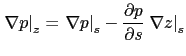
in ![]() -coordinate consists of two terms (see Appendix A),
-coordinate consists of two terms (see Appendix A),
The second term in (2.33) depends on the tilt of the coordinate surface
and introduces a truncation error that is not present in a ![]() -model. In the special case
of a
-model. In the special case
of a ![]() coordinate (i.e. a depth-normalised coordinate system
coordinate (i.e. a depth-normalised coordinate system
![]() ),
Haney [1991] and Beckmann and Haidvogel [1993] have given estimates of the magnitude
of this truncation error. It depends on topographic slope, stratification, horizontal and
vertical resolution, the equation of state, and the finite difference scheme. This error
limits the possible topographic slopes that a model can handle at a given horizontal
and vertical resolution. This is a severe restriction for large-scale applications using
realistic bottom topography. The large-scale slopes require high horizontal resolution,
and the computational cost becomes prohibitive. This problem can be at least partially
overcome by mixing
),
Haney [1991] and Beckmann and Haidvogel [1993] have given estimates of the magnitude
of this truncation error. It depends on topographic slope, stratification, horizontal and
vertical resolution, the equation of state, and the finite difference scheme. This error
limits the possible topographic slopes that a model can handle at a given horizontal
and vertical resolution. This is a severe restriction for large-scale applications using
realistic bottom topography. The large-scale slopes require high horizontal resolution,
and the computational cost becomes prohibitive. This problem can be at least partially
overcome by mixing ![]() -coordinate and step-like representation of bottom topography [Gerdes, 1993b, Gerdes, 1993a, Madec et al., 1996]. However, the definition of the model
domain vertical coordinate becomes then a non-trivial thing for a realistic bottom
topography: a envelope topography is defined in
-coordinate and step-like representation of bottom topography [Gerdes, 1993b, Gerdes, 1993a, Madec et al., 1996]. However, the definition of the model
domain vertical coordinate becomes then a non-trivial thing for a realistic bottom
topography: a envelope topography is defined in ![]() -coordinate on which a full or
partial step bottom topography is then applied in order to adjust the model depth to
the observed one (see §4.3.
-coordinate on which a full or
partial step bottom topography is then applied in order to adjust the model depth to
the observed one (see §4.3.
For numerical reasons a minimum of diffusion is required along the coordinate surfaces
of any finite difference model. It causes spurious diapycnal mixing when coordinate
surfaces do not coincide with isoneutral surfaces. This is the case for a ![]() -model as
well as for a
-model as
well as for a ![]() -model. However, density varies more strongly on
-model. However, density varies more strongly on ![]() surfaces than
on horizontal surfaces in regions of large topographic slopes, implying larger diapycnal
diffusion in a
surfaces than
on horizontal surfaces in regions of large topographic slopes, implying larger diapycnal
diffusion in a ![]() -model than in a
-model than in a ![]() -model. Whereas such a diapycnal diffusion in a
-model. Whereas such a diapycnal diffusion in a
![]() -model tends to weaken horizontal density (pressure) gradients and thus the horizontal
circulation, it usually reinforces these gradients in a
-model tends to weaken horizontal density (pressure) gradients and thus the horizontal
circulation, it usually reinforces these gradients in a ![]() -model, creating spurious circulation.
For example, imagine an isolated bump of topography in an ocean at rest with a horizontally
uniform stratification. Spurious diffusion along
-model, creating spurious circulation.
For example, imagine an isolated bump of topography in an ocean at rest with a horizontally
uniform stratification. Spurious diffusion along ![]() -surfaces will induce a bump of isoneutral
surfaces over the topography, and thus will generate there a baroclinic eddy. In contrast,
the ocean will stay at rest in a
-surfaces will induce a bump of isoneutral
surfaces over the topography, and thus will generate there a baroclinic eddy. In contrast,
the ocean will stay at rest in a ![]() -model. As for the truncation error, the problem can be reduced by introducing the terrain-following coordinate below the strongly stratified portion of the water column
(
-model. As for the truncation error, the problem can be reduced by introducing the terrain-following coordinate below the strongly stratified portion of the water column
(![]() the main thermocline) [Madec et al., 1996]. An alternate solution consists of rotating
the lateral diffusive tensor to geopotential or to isoneutral surfaces (see §2.5.2.
Unfortunately, the slope of isoneutral surfaces relative to the
the main thermocline) [Madec et al., 1996]. An alternate solution consists of rotating
the lateral diffusive tensor to geopotential or to isoneutral surfaces (see §2.5.2.
Unfortunately, the slope of isoneutral surfaces relative to the ![]() -surfaces can very large,
strongly exceeding the stability limit of such a operator when it is discretized (see Chapter 9).
-surfaces can very large,
strongly exceeding the stability limit of such a operator when it is discretized (see Chapter 9).
The ![]() coordinates introduced here [Madec et al., 1996, Lott et al., 1990] differ mainly in two
aspects from similar models: it allows a representation of bottom topography with mixed
full or partial step-like/terrain following topography ; It also offers a completely general
transformation,
coordinates introduced here [Madec et al., 1996, Lott et al., 1990] differ mainly in two
aspects from similar models: it allows a representation of bottom topography with mixed
full or partial step-like/terrain following topography ; It also offers a completely general
transformation,
![]() for the vertical coordinate.
for the vertical coordinate.
The ![]() -coordinate has been developed by Leclair and Madec [2011].
It is available in NEMO since the version 3.4. Nevertheless, it is currently not robust enough
to be used in all possible configurations. Its use is therefore not recommended.
-coordinate has been developed by Leclair and Madec [2011].
It is available in NEMO since the version 3.4. Nevertheless, it is currently not robust enough
to be used in all possible configurations. Its use is therefore not recommended.
Gurvan Madec and the NEMO Team
NEMO European Consortium2017-02-17
 , and
, and 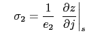

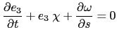 with
with ![$\displaystyle \;\; \chi =\frac{1}{e_1 e_2 e_3 }\left[ {\frac{\partial \left( {e...
...}{\partial i}+\frac{\partial \left( {e_1 e_3 v} \right)}{\partial j}} \right]$](img207.png)