Direction of Lateral Mixing (ldfslp.F90)

A direction for lateral mixing has to be defined when the desired operator does not act along the model levels. This occurs when $(a)$ horizontal mixing is required on tracer or momentum (ln_traldf_hor or ln_dynldf_hor) in $s$- or mixed $s$-$z$- coordinates, and $(b)$ isoneutral mixing is required whatever the vertical coordinate is. This direction of mixing is defined by its slopes in the i- and j-directions at the face of the cell of the quantity to be diffused. For a tracer, this leads to the following four slopes : $r_{1u}$, $r_{1w}$, $r_{2v}$, $r_{2w}$ (see (5.9)), while for momentum the slopes are $r_{1t}$, $r_{1uw}$, $r_{2f}$, $r_{2uw}$ for $u$ and $r_{1f}$, $r_{1vw}$, $r_{2t}$, $r_{2vw}$ for $v$.

slopes for tracer geopotential mixing in the $s$-coordinate

In $s$-coordinates, geopotential mixing ($i.e.$ horizontal mixing) $r_1$ and $r_2$ are the slopes between the geopotential and computational surfaces. Their discrete formulation is found by locally solving (5.9) when the diffusive fluxes in the three directions are set to zero and $T$ is assumed to be horizontally uniform, $i.e.$ a linear function of $z_T$, the depth of a $T$-point.

$$\begin{aligned}r_{1u} &= \frac{e_{3u}}{ \left( e_{1u}\;\overlin... ...approx \frac{1}{e_{2w}}\; \delta_{j+1/2}[z_{vw}] \end{aligned}$$

These slopes are computed once in ldfslp_init when ln_sco=True, and either ln_traldf_hor=True or ln_dynldf_hor=True.

Slopes for tracer iso-neutral mixing

In iso-neutral mixing $r_1$ and $r_2$ are the slopes between the iso-neutral and computational surfaces. Their formulation does not depend on the vertical coordinate used. Their discrete formulation is found using the fact that the diffusive fluxes of locally referenced potential density ($i.e.$ $in situ$ density) vanish. So, substituting $T$ by $\rho$ in (5.9) and setting the diffusive fluxes in the three directions to zero leads to the following definition for the neutral slopes:

$$\begin{split}r_{1u} &= \frac{e_{3u}}{e_{1u}}\; \frac{\delta_{... ...2}[\rho]}}^{ j, k+1/2}} {\delta_{k+1/2}[\rho]} \end{split}$$ (9.11)

As the mixing is performed along neutral surfaces, the gradient of $\rho$ in (9.11) has to be evaluated at the same local pressure (which, in decibars, is approximated by the depth in meters in the model). Therefore (9.11) cannot be used as such, but further transformation is needed depending on the vertical coordinate used:

$z$-coordinate with full step :

in (9.11) the densities appearing in the $i$ and $j$ derivatives are taken at the same depth, thus the $in situ$ density can be used. This is not the case for the vertical derivatives: $\delta_{k+1/2}[\rho]$ is replaced by $-\rho N^2/g$, where $N^2$ is the local Brunt-Vaisälä frequency evaluated following McDougall [1987] (see §5.8.2).

$z$-coordinate with partial step :

this case is identical to the full step case except that at partial step level, the horizontal density gradient is evaluated as described in §5.9.

$s$- or hybrid $s$-$z$- coordinate :

in the current release of NEMO, iso-neutral mixing is only employed for $s$-coordinates if the Griffies scheme is used (traldf_grif=true; see Appdx D). In other words, iso-neutral mixing will only be accurately represented with a linear equation of state (nn_eos=1 or 2). In the case of a "true" equation of state, the evaluation of $i$ and $j$ derivatives in (9.11) will include a pressure dependent part, leading to the wrong evaluation of the neutral slopes.

Note: The solution for $s$-coordinate passes trough the use of different (and better) expression for the constraint on iso-neutral fluxes. Following Griffies [2004], instead of specifying directly that there is a zero neutral diffusive flux of locally referenced potential density, we stay in the $T$-$S$ plane and consider the balance between the neutral direction diffusive fluxes of potential temperature and salinity:

$$\alpha \textbf{F}(T) = \beta \textbf{F}(S)$$ (9.12)

This constraint leads to the following definition for the slopes:

$$\begin{split}r_{1u} &= \frac{e_{3u}}{e_{1u}}\; \frac {\alpha_... ...\delta_{k+1/2}[T] - \beta_w \;\delta_{k+1/2}[S]} \end{split}$$ (9.13)

where $\alpha$ and $\beta$, the thermal expansion and saline contraction coefficients introduced in §5.8.2, have to be evaluated at the three velocity points. In order to save computation time, they should be approximated by the mean of their values at $T$-points (for example in the case of $\alpha$: $\alpha_u=\overline{\alpha_T}^{i+1/2}$, $\alpha_v=\overline{\alpha_T}^{j+1/2}$ and $\alpha_w=\overline{\alpha_T}^{k+1/2}$).

Note that such a formulation could be also used in the $z$-coordinate and $z$-coordinate with partial steps cases.

This implementation is a rather old one. It is similar to the one proposed by Cox [1987], except for the background horizontal diffusion. Indeed, the Cox implementation of isopycnal diffusion in GFDL-type models requires a minimum background horizontal diffusion for numerical stability reasons. To overcome this problem, several techniques have been proposed in which the numerical schemes of the ocean model are modified [Weaver and Eby, 1997, Griffies et al., 1998]. Griffies's scheme is now available in NEMO if traldf_grif_iso is set true; see Appdx D. Here, another strategy is presented [Lazar, 1997]: a local filtering of the iso-neutral slopes (made on 9 grid-points) prevents the development of grid point noise generated by the iso-neutral diffusion operator (Fig. 9.1). This allows an iso-neutral diffusion scheme without additional background horizontal mixing. This technique can be viewed as a diffusion operator that acts along large-scale (2 $\Delta$x) iso-neutral surfaces. The diapycnal diffusion required for numerical stability is thus minimized and its net effect on the flow is quite small when compared to the effect of an horizontal background mixing.

Nevertheless, this iso-neutral operator does not ensure that variance cannot increase, contrary to the Griffies et al. [1998] operator which has that property.

Figure 9.1: averaging procedure for isopycnal slope computation.

For numerical stability reasons [Griffies, 2004, Cox, 1987], the slopes must also be bounded by $1/100$ everywhere. This constraint is applied in a piecewise linear fashion, increasing from zero at the surface to $1/100$ at $70$ metres and thereafter decreasing to zero at the bottom of the ocean. (the fact that the eddies "feel" the surface motivates this flattening of isopycnals near the surface).

Figure 9.2: Vertical profile of the slope used for lateral mixing in the mixed layer : (a) in the real ocean the slope is the iso-neutral slope in the ocean interior, which has to be adjusted at the surface boundary (i.e. it must tend to zero at the surface since there is no mixing across the air-sea interface: wall boundary condition). Nevertheless, the profile between the surface zero value and the interior iso-neutral one is unknown, and especially the value at the base of the mixed layer ; (b) profile of slope using a linear tapering of the slope near the surface and imposing a maximum slope of 1/100 ; (c) profile of slope actually used in NEMO: a linear decrease of the slope from zero at the surface to its ocean interior value computed just below the mixed layer. Note the huge change in the slope at the base of the mixed layer between (b) and (c).

yellowadd here a discussion about the flattening of the slopes, vs tapering the coefficient.

slopes for momentum iso-neutral mixing

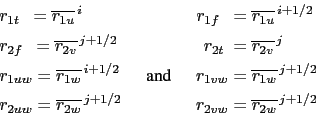
The iso-neutral diffusion operator on momentum is the same as the one used on tracers but applied to each component of the velocity separately (see (6.27) in section 6.6.2). The slopes between the surface along which the diffusion operator acts and the surface of computation ($z$- or $s$-surfaces) are defined at $T$-, $f$-, and uw- points for the $u$-component, and $T$-, $f$- and vw- points for the $v$-component. They are computed from the slopes used for tracer diffusion, $i.e.$ (9.10) and (9.11) :

$$\begin{aligned}&r_{1t} = \overline{r_{1u}}^{ i} &&& r_{1f}\... ...,j+1/2} &&& r_{2vw}&= \overline{r_{2w}}^{ j+1/2} \end{aligned}$$

The major issue remaining is in the specification of the boundary conditions. The same boundary conditions are chosen as those used for lateral diffusion along model level surfaces, i.e. using the shear computed along the model levels and with no additional friction at the ocean bottom (see §8.1).