Next: Direction of Lateral Mixing Up: Lateral Ocean Physics (LDF) Previous: Lateral Ocean Physics (LDF) Contents Index
Introducing a space variation in the lateral eddy mixing coefficients changes the model core memory requirement, adding up to four extra three-dimensional arrays for the geopotential or isopycnal second order operator applied to momentum. Six CPP keys control the space variation of eddy coefficients: three for momentum and three for tracer. The three choices allow: a space variation in the three space directions (key_ traldf_c3d, key_ dynldf_c3d), in the horizontal plane (key_ traldf_c2d, key_ dynldf_c2d), or in the vertical only (key_ traldf_c1d, key_ dynldf_c1d). The default option is a constant value over the whole ocean on both momentum and tracers.
The number of additional arrays that have to be defined and the gridpoint position at which they are defined depend on both the space variation chosen and the type of operator used. The resulting eddy viscosity and diffusivity coefficients can be a function of more than one variable. Changes in the computer code when switching from one option to another have been minimized by introducing the eddy coefficients as statement functions (include file ldftra_substitute.h90 and ldfdyn_substitute.h90). The functions are replaced by their actual meaning during the preprocessing step (CPP). The specification of the space variation of the coefficient is made in ldftra.F90 and ldfdyn.F90, or more precisely in include files traldf_cNd.h90 and dynldf_cNd.h90, with N=1, 2 or 3. The user can modify these include files as he/she wishes. The way the mixing coefficient are set in the reference version can be briefly described as follows:
Other formulations can be introduced by the user for a given configuration.
For example, in the ORCA2 global ocean model (see Configurations), the laplacian
viscosity operator uses rn_ahm_0_lap = 4.10![]() m
m![]() /s poleward of 20
north and south and decreases linearly to rn_aht_0 = 2.10
/s poleward of 20
north and south and decreases linearly to rn_aht_0 = 2.10![]() m
m![]() /s
at the equator [Delecluse and Madec, 2000, Madec et al., 1996]. This modification
can be found in routine ldf_dyn_c2d_orca defined in ldfdyn_c2d.F90.
Similar modified horizontal variations can be found with the Antarctic or Arctic
sub-domain options of ORCA2 and ORCA05 (see &namcfg namelist).
/s
at the equator [Delecluse and Madec, 2000, Madec et al., 1996]. This modification
can be found in routine ldf_dyn_c2d_orca defined in ldfdyn_c2d.F90.
Similar modified horizontal variations can be found with the Antarctic or Arctic
sub-domain options of ORCA2 and ORCA05 (see &namcfg namelist).
The 3D space variation of the mixing coefficient is simply the combination of the
1D and 2D cases, ![]() a hyperbolic tangent variation with depth associated with
a grid size dependence of the magnitude of the coefficient.
a hyperbolic tangent variation with depth associated with
a grid size dependence of the magnitude of the coefficient.
There are no default specifications of space and time varying mixing coefficient. One available case is specific to the ORCA2 and ORCA05 global ocean configurations. It provides only a tracer mixing coefficient for eddy induced velocity (ORCA2) or both iso-neutral and eddy induced velocity (ORCA05) that depends on the local growth rate of baroclinic instability. This specification is actually used when an ORCA key and both key_ traldf_eiv and key_ traldf_c2d are defined.
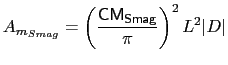
The key_ dynldf_smag key activates a 3D, time-varying viscosity that depends on the resolved motions. Following [Smagorinsky, 1993] the viscosity coefficient is set proportional to a local deformation rate based on the horizontal shear and tension, namely:
 |
(9.2) |
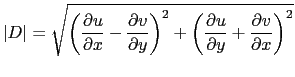
where the deformation rate
![]() is given by
is given by
 |
(9.3) |
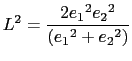
and ![]() is the local gridscale given by:
is the local gridscale given by:
 |
(9.4) |
[Griffies and Hallberg, 2000] suggest values in the range 2.2 to 4.0 of the coefficient
![]() for oceanic flows. This value is set via the rn_cmsmag_1 namelist
parameter. An additional parameter: rn_cmsh is included in NEMO for experimenting
with the contribution of the shear term. A value of 1.0 (the default) calculates the
deformation rate as above; a value of 0.0 will discard the shear term entirely.
for oceanic flows. This value is set via the rn_cmsmag_1 namelist
parameter. An additional parameter: rn_cmsh is included in NEMO for experimenting
with the contribution of the shear term. A value of 1.0 (the default) calculates the
deformation rate as above; a value of 0.0 will discard the shear term entirely.
For numerical stability, the calculated viscosity is bounded according to the following:
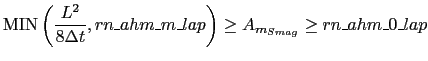 |
(9.5) |
with both parameters for the upper and lower bounds being provided via the indicated namelist parameters.
When
![]() , a biharmonic version of the Smagorinsky
viscosity is also available which sets a coefficient for the biharmonic viscosity as:
, a biharmonic version of the Smagorinsky
viscosity is also available which sets a coefficient for the biharmonic viscosity as:
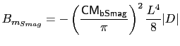 |
(9.6) |
which is bounded according to:
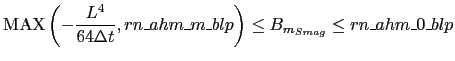 |
(9.7) |
Note the reversal of the inequalities here because NEMO requires the biharmonic
coefficients as negative numbers.
![]() is set via the rn_cmsmag_2
namelist parameter and the bounding values have corresponding entries in the namelist too.
is set via the rn_cmsmag_2
namelist parameter and the bounding values have corresponding entries in the namelist too.
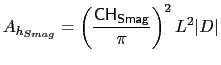
The current implementation in NEMO also allows for 3D, time-varying diffusivities
to be set using the Smagorinsky approach. Users should note that this option is not
recommended for many applications since diffusivities will tend to be largest near
boundaries (where shears are greatest) leading to spurious upwellings
([Griffies, 2004], chapter 18.3.4). Nevertheless the option is there for those
wishing to experiment. This choice requires both key_ traldf_c3d and key_ traldf_smag
and uses the rn_chsmag (
![]() ), rn_smsh and rn_aht_m
namelist parameters in an analogous way to rn_cmsmag_1, rn_cmsh and
rn_ahm_m_lap (see above) to set the diffusion coefficient:
), rn_smsh and rn_aht_m
namelist parameters in an analogous way to rn_cmsmag_1, rn_cmsh and
rn_ahm_m_lap (see above) to set the diffusion coefficient:
 |
(9.8) |
For numerical stability, the calculated diffusivity is bounded according to the following:
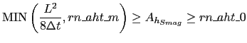 |
(9.9) |
![]()
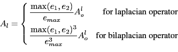
The following points are relevant when the eddy coefficient varies spatially:
(1) the momentum diffusion operator acting along model level surfaces is written in terms of curl and divergent components of the horizontal current (see §2.5.2). Although the eddy coefficient could be set to different values in these two terms, this option is not currently available.
(2) with an horizontally varying viscosity, the quadratic integral constraints on enstrophy and on the square of the horizontal divergence for operators acting along model-surfaces are no longer satisfied (Appendix C.7).
(3) for isopycnal diffusion on momentum or tracers, an additional purely horizontal background diffusion with uniform coefficient can be added by setting a non zero value of rn_ahmb_0 or rn_ahtb_0, a background horizontal eddy viscosity or diffusivity coefficient (namelist parameters whose default values are 0). However, the technique used to compute the isopycnal slopes is intended to get rid of such a background diffusion, since it introduces spurious diapycnal diffusion (see §9.2).
(4) when an eddy induced advection term is used (key_ traldf_eiv), ![]() ,
the eddy induced coefficient has to be defined. Its space variations are controlled
by the same CPP variable as for the eddy diffusivity coefficient (
,
the eddy induced coefficient has to be defined. Its space variations are controlled
by the same CPP variable as for the eddy diffusivity coefficient (![]() key_traldf_cNd).
key_traldf_cNd).
(5) the eddy coefficient associated with a biharmonic operator must be set to a negative value.
(6) it is possible to use both the laplacian and biharmonic operators concurrently.
(7) it is possible to run without explicit lateral diffusion on momentum (ln_dynldf_lap = ln_dynldf_bilap = false). This is recommended when using the UBS advection scheme on momentum (ln_dynadv_ubs = true, see 6.3.2) and can be useful for testing purposes.
Gurvan Madec and the NEMO Team
NEMO European Consortium2017-02-17