Next: Hydrostatic Pressure Gradient Up: Time Domain (STP) Previous: Non-Diffusive Part Contents Index
The leapfrog differencing scheme is unsuitable for the representation of
diffusion and damping processes. For a tendancy ![]() , representing a
diffusion term or a restoring term to a tracer climatology
(when present, see § 5.6), a forward time differencing scheme
is used :
, representing a
diffusion term or a restoring term to a tracer climatology
(when present, see § 5.6), a forward time differencing scheme
is used :
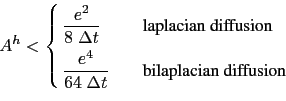
This is diffusive in time and conditionally stable. The conditions for stability of second and fourth order horizontal diffusion schemes are [Griffies, 2004]:
For the vertical diffusion terms, a forward time differencing scheme can be
used, but usually the numerical stability condition imposes a strong
constraint on the time step. Two solutions are available in NEMO to overcome
the stability constraint: ![]() a forward time differencing scheme using a
time splitting technique (ln_zdfexp = true) or
a forward time differencing scheme using a
time splitting technique (ln_zdfexp = true) or ![]() a backward (or implicit)
time differencing scheme (ln_zdfexp = false). In
a backward (or implicit)
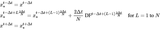
time differencing scheme (ln_zdfexp = false). In ![]() , the master
time step
, the master
time step ![]() t is cut into
t is cut into ![]() fractional time steps so that the
stability criterion is reduced by a factor of
fractional time steps so that the
stability criterion is reduced by a factor of ![]() . The computation is performed as
follows:
. The computation is performed as
follows:
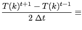
This scheme is rather time consuming since it requires a matrix inversion, but it becomes attractive since a value of 3 or more is needed for N in the forward time differencing scheme. For example, the finite difference approximation of the temperature equation is:
(3.8) is a linear system of equations with an associated
matrix which is tridiagonal. Moreover, ![]() and
and ![]() are positive and the diagonal
term is greater than the sum of the two extra-diagonal terms, therefore a special
adaptation of the Gauss elimination procedure is used to find the solution
(see for example Richtmyer and Morton [1967]).
are positive and the diagonal
term is greater than the sum of the two extra-diagonal terms, therefore a special
adaptation of the Gauss elimination procedure is used to find the solution
(see for example Richtmyer and Morton [1967]).
Gurvan Madec and the NEMO Team
NEMO European Consortium2017-02-17
 RHS
RHS![$\displaystyle +\frac{1}{e_{3t} }\delta _k \left[ {\frac{A_w^{vT} }{e_{3w} }\delta _{k+1/2} \left[ {T^{t+1}} \right]} \right]$](img287.png)