Equation of State (eosbn2.F90)

!-----------------------------------------------------------------------
&nameos        !   ocean physical parameters
!-----------------------------------------------------------------------
   nn_eos      =  -1     !  type of equation of state and Brunt-Vaisala frequency
                                 !  =-1, TEOS-10
                                 !  = 0, EOS-80
                                 !  = 1, S-EOS   (simplified eos)
   ln_useCT    = .true.  ! use of Conservative Temp. ==> surface CT converted in Pot. Temp. in sbcssm
   !                             !
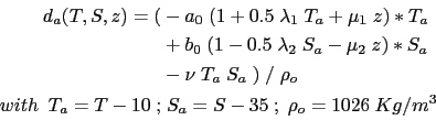
   !                     ! S-EOS coefficients :
   !                             !  rd(T,S,Z)*rau0 = -a0*(1+.5*lambda*dT+mu*Z+nu*dS)*dT+b0*dS
   rn_a0       =  1.6550e-1      !  thermal expension coefficient (nn_eos= 1)
   rn_b0       =  7.6554e-1      !  saline  expension coefficient (nn_eos= 1)
   rn_lambda1  =  5.9520e-2      !  cabbeling coeff in T^2  (=0 for linear eos)
   rn_lambda2  =  7.4914e-4      !  cabbeling coeff in S^2  (=0 for linear eos)
   rn_mu1      =  1.4970e-4      !  thermobaric coeff. in T (=0 for linear eos)
   rn_mu2      =  1.1090e-5      !  thermobaric coeff. in S (=0 for linear eos)
   rn_nu       =  2.4341e-3      !  cabbeling coeff in T*S  (=0 for linear eos)
/

Equation Of Seawater (nn_eos = -1, 0, or 1)

The Equation Of Seawater (EOS) is an empirical nonlinear thermodynamic relationship linking seawater density, $\rho$, to a number of state variables, most typically temperature, salinity and pressure. Because density gradients control the pressure gradient force through the hydrostatic balance, the equation of state provides a fundamental bridge between the distribution of active tracers and the fluid dynamics. Nonlinearities of the EOS are of major importance, in particular influencing the circulation through determination of the static stability below the mixed layer, thus controlling rates of exchange between the atmosphere and the ocean interior [Roquet et al., 2015a]. Therefore an accurate EOS based on either the 1980 equation of state (EOS-80, UNESCO [1983]) or TEOS-10 [IOC et al., 2010] standards should be used anytime a simulation of the real ocean circulation is attempted [Roquet et al., 2015a]. The use of TEOS-10 is highly recommended because (i) it is the new official EOS, (ii) it is more accurate, being based on an updated database of laboratory measurements, and (iii) it uses Conservative Temperature and Absolute Salinity (instead of potential temperature and practical salinity for EOS-980, both variables being more suitable for use as model variables [Graham and McDougall, 2013, IOC et al., 2010]. EOS-80 is an obsolescent feature of the NEMO system, kept only for backward compatibility. For process studies, it is often convenient to use an approximation of the EOS. To that purposed, a simplified EOS (S-EOS) inspired by Vallis [2006] is also available.

In the computer code, a density anomaly, $d_a= \rho / \rho_o - 1$, is computed, with $\rho_o$ a reference density. Called rau0 in the code, $\rho_o$ is set in phycst.F90 to a value of $1,026 Kg/m^3$. This is a sensible choice for the reference density used in a Boussinesq ocean climate model, as, with the exception of only a small percentage of the ocean, density in the World Ocean varies by no more than 2$\%$ from that value [Gill, 1982].

Options are defined through the nameos namelist variables, and in particular nn_eos which controls the EOS used (=-1 for TEOS10 ; =0 for EOS-80 ; =1 for S-EOS).

nn_eos$=-1$

the polyTEOS10-bsq equation of seawater [Roquet et al., 2015b] is used. The accuracy of this approximation is comparable to the TEOS-10 rational function approximation, but it is optimized for a boussinesq fluid and the polynomial expressions have simpler and more computationally efficient expressions for their derived quantities which make them more adapted for use in ocean models. Note that a slightly higher precision polynomial form is now used replacement of the TEOS-10 rational function approximation for hydrographic data analysis [IOC et al., 2010]. A key point is that conservative state variables are used: Absolute Salinity (unit: g/kg, notation: $S_A$) and Conservative Temperature (unit: , notation: $\Theta$). The pressure in decibars is approximated by the depth in meters. With TEOS10, the specific heat capacity of sea water, $C_p$, is a constant. It is set to $C_p=3991.86795711963 J Kg^{-1} ^{\circ}K^{-1}$, according to IOC et al. [2010].

Choosing polyTEOS10-bsq implies that the state variables used by the model are $\Theta$ and $S_A$. In particular, the initial state deined by the user have to be given as Conservative Temperature and Absolute Salinity. In addition, setting ln_useCT to true convert the Conservative SST to potential SST prior to either computing the air-sea and ice-sea fluxes (forced mode) or sending the SST field to the atmosphere (coupled mode).

nn_eos$=0$

the polyEOS80-bsq equation of seawater is used. It takes the same polynomial form as the polyTEOS10, but the coefficients have been optimized to accurately fit EOS80 (Roquet, personal comm.). The state variables used in both the EOS80 and the ocean model are: the Practical Salinity ((unit: psu, notation: $S_p$)) and Potential Temperature (unit: $^{\circ}C$, notation: $\theta$). The pressure in decibars is approximated by the depth in meters. With thsi EOS, the specific heat capacity of sea water, $C_p$, is a function of temperature, salinity and pressure [UNESCO, 1983]. Nevertheless, a severe assumption is made in order to have a heat content ($C_p T_p$) which is conserved by the model: $C_p$ is set to a constant value, the TEOS10 value.

nn_eos$=1$

a simplified EOS (S-EOS) inspired by Vallis [2006] is chosen, the coefficients of which has been optimized to fit the behavior of TEOS10 (Roquet, personal comm.) (see also Roquet et al. [2015a]). It provides a simplistic linear representation of both cabbeling and thermobaricity effects which is enough for a proper treatment of the EOS in theoretical studies [Roquet et al., 2015a]. With such an equation of state there is no longer a distinction between conservative and potential temperature, as well as between absolute and practical salinity. S-EOS takes the following expression:

$$\begin{split}d_a(T,S,z) = ( & - a_0 \; ( 1 + 0.5 \; \lambda_1... ...10 \; ; & \; S_a = S-35 \; ;\; \rho_o = 1026 Kg/m^3 \end{split}$$ (5.25)

where the computer name of the coefficients as well as their standard value are given in 5.1. In fact, when choosing S-EOS, various approximation of EOS can be specified simply by changing the associated coefficients. Setting to zero the two thermobaric coefficients ($\mu_1$, $\mu_2$) remove thermobaric effect from S-EOS. setting to zero the three cabbeling coefficients ($\lambda_1$, $\lambda_2$, $\nu$) remove cabbeling effect from S-EOS. Keeping non-zero value to $a_0$ and $b_0$ provide a linear EOS function of T and S.

Table 5.1: Standard value of S-EOS coefficients.

coeff.	computer name	S-EOS	description
$a_0$	rn_a0	1.6550 $10^{-1}$	linear thermal expansion coeff.
$b_0$	rn_b0	7.6554 $10^{-1}$	linear haline expansion coeff.
$\lambda_1$	rn_lambda1	5.9520 $10^{-2}$	cabbeling coeff. in $T^2$
$\lambda_2$	rn_lambda2	5.4914 $10^{-4}$	cabbeling coeff. in $S^2$
$\nu$	rn_nu	2.4341 $10^{-3}$	cabbeling coeff. in $T S$
$\mu_1$	rn_mu1	1.4970 $10^{-4}$	thermobaric coeff. in T
$\mu_2$	rn_mu2	1.1090 $10^{-5}$	thermobaric coeff. in S

Brunt-Väisälä Frequency (nn_eos = 0, 1 or 2)

An accurate computation of the ocean stability (i.e. of $N$, the brunt-Väisälä frequency) is of paramount importance as determine the ocean stratification and is used in several ocean parameterisations (namely TKE, GLS, Richardson number dependent vertical diffusion, enhanced vertical diffusion, non-penetrative convection, tidal mixing parameterisation, iso-neutral diffusion). In particular, $N^2$ has to be computed at the local pressure (pressure in decibar being approximated by the depth in meters). The expression for $N^2$ is given by:

$$N^2 = \frac{g}{e_{3w}} \left( \beta \;\delta_{k+1/2}[S] - \alpha \;\delta_{k+1/2}[T] \right)$$ (5.26)

where $(T,S) = (\Theta, S_A)$ for TEOS10, $= (\theta, S_p)$ for TEOS-80, or $=(T,S)$ for S-EOS, and, $\alpha$ and $\beta$ are the thermal and haline expansion coefficients. The coefficients are a polynomial function of temperature, salinity and depth which expression depends on the chosen EOS. They are computed through eos_rab, a FORTRAN function that can be found in eosbn2.F90.

Freezing Point of Seawater

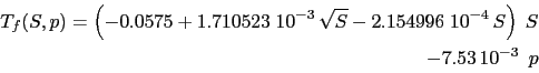
The freezing point of seawater is a function of salinity and pressure [UNESCO, 1983]:

$$\begin{split}T_f (S,p) = \left( -0.0575 + 1.710523 \;10^{-3} ... ... \;10^{-4} S \right) S - 7.53 10^{-3} p \end{split}$$ (5.27)

(5.27) is only used to compute the potential freezing point of sea water ($i.e.$ referenced to the surface $p=0$), thus the pressure dependent terms in (5.27) (last term) have been dropped. The freezing point is computed through eos_fzp, a FORTRAN function that can be found in eosbn2.F90.