Next: Domain: Initial State (istate Up: Space Domain (DOM) Previous: Domain: Horizontal Grid (mesh) Contents Index
!-----------------------------------------------------------------------
&namzgr        !   vertical coordinate
!-----------------------------------------------------------------------
   ln_zco      = .false.   !  z-coordinate - full    steps   (T/F)      ("key_zco" may also be defined)
   ln_zps      = .true.    !  z-coordinate - partial steps   (T/F)
   ln_sco      = .false.   !  s- or hybrid z-s-coordinate    (T/F)
   ln_isfcav   = .false.   !  ice shelf cavity               (T/F)
/
!-----------------------------------------------------------------------
&namdom        !   space and time domain (bathymetry, mesh, timestep)
!-----------------------------------------------------------------------
   nn_bathy    =    1      !  compute (=0) or read (=1) the bathymetry file
   rn_bathy    =    0.     !  value of the bathymetry. if (=0) bottom flat at jpkm1
   nn_closea   =    0      !  remove (=0) or keep (=1) closed seas and lakes (ORCA)
   nn_msh      =    1      !  create (=1) a mesh file or not (=0)
   rn_hmin     =   -3.     !  min depth of the ocean (>0) or min number of ocean level (<0)
   rn_e3zps_min=   20.     !  partial step thickness is set larger than the minimum of
   rn_e3zps_rat=    0.1    !  rn_e3zps_min and rn_e3zps_rat*e3t, with 0<rn_e3zps_rat<1
                           !
   rn_rdt      = 5760.     !  time step for the dynamics (and tracer if nn_acc=0)
   rn_atfp     =    0.1    !  asselin time filter parameter
   nn_acc      =    0      !  acceleration of convergence : =1      used, rdt < rdttra(k)
                                 !                          =0, not used, rdt = rdttra
   rn_rdtmin   = 28800.          !  minimum time step on tracers (used if nn_acc=1)
   rn_rdtmax   = 28800.          !  maximum time step on tracers (used if nn_acc=1)
   rn_rdth     =  800.           !  depth variation of tracer time step  (used if nn_acc=1)
   ln_crs      = .false.      !  Logical switch for coarsening module
   jphgr_msh   =       0               !  type of horizontal mesh
                                       !  = 0 curvilinear coordinate on the sphere read in coordinate.nc
                                       !  = 1 geographical mesh on the sphere with regular grid-spacing
                                       !  = 2 f-plane with regular grid-spacing
                                       !  = 3 beta-plane with regular grid-spacing
                                       !  = 4 Mercator grid with T/U point at the equator
   ppglam0     =       0.0             !  longitude of first raw and column T-point (jphgr_msh = 1)
   ppgphi0     =     -35.0             ! latitude  of first raw and column T-point (jphgr_msh = 1)
   ppe1_deg    =       1.0             !  zonal      grid-spacing (degrees)
   ppe2_deg    =       0.5             !  meridional grid-spacing (degrees)
   ppe1_m      =    5000.0             !  zonal      grid-spacing (degrees)
   ppe2_m      =    5000.0             !  meridional grid-spacing (degrees)
   ppsur       =    -4762.96143546300  !  ORCA r4, r2 and r05 coefficients
   ppa0        =      255.58049070440  ! (default coefficients)
   ppa1        =      245.58132232490  !
   ppkth       =       21.43336197938  !
   ppacr       =        3.0            !
   ppdzmin     =       10.             !  Minimum vertical spacing
   pphmax      =     5000.             !  Maximum depth
   ldbletanh   =    .TRUE.             !  Use/do not use double tanf function for vertical coordinates
   ppa2        =      100.760928500000 !  Double tanh function parameters
   ppkth2      =       48.029893720000 !
   ppacr2      =       13.000000000000 !
/
Variables are defined through the namzgr and namdom namelists.
In the vertical, the model mesh is determined by four things:
(1) the bathymetry given in meters ;
(2) the number of levels of the model (jpk) ;
(3) the analytical transformation ![]() and the vertical scale factors
(derivatives of the transformation) ;
and (4) the masking system,
and the vertical scale factors
(derivatives of the transformation) ;
and (4) the masking system, ![]() the number of wet model levels at each
the number of wet model levels at each
![]() column of points.
column of points.
The choice of a vertical coordinate, even if it is made through namzgr namelist parameters,
must be done once of all at the beginning of an experiment. It is not intended as an
option which can be enabled or disabled in the middle of an experiment. Three main
choices are offered (Fig. 4.5a to c): ![]() -coordinate with full step
bathymetry (ln_zco = true),
-coordinate with full step
bathymetry (ln_zco = true), ![]() -coordinate with partial step bathymetry
(ln_zps = true), or generalized,
-coordinate with partial step bathymetry
(ln_zps = true), or generalized, ![]() -coordinate (ln_sco = true).
Hybridation of the three main coordinates are available:
-coordinate (ln_sco = true).
Hybridation of the three main coordinates are available: ![]() or
or ![]() coordinate
(Fig. 4.5d and 4.5e). When using the variable
volume option key_ vvl (
coordinate
(Fig. 4.5d and 4.5e). When using the variable
volume option key_ vvl (![]() non-linear free surface), the coordinate follow the
time-variation of the free surface so that the transformation is time dependent:
non-linear free surface), the coordinate follow the
time-variation of the free surface so that the transformation is time dependent:
![]() (Fig. 4.5f). This option can be used with full step
bathymetry or
(Fig. 4.5f). This option can be used with full step
bathymetry or ![]() -coordinate (hybrid and partial step coordinates have not
yet been tested in NEMO v2.3). If using
-coordinate (hybrid and partial step coordinates have not
yet been tested in NEMO v2.3). If using ![]() -coordinate with partial step bathymetry
(ln_zps = true), ocean cavity beneath ice shelves can be open (ln_isfcav = true)
and partial step are also applied at the ocean/ice shelf interface.
-coordinate with partial step bathymetry
(ln_zps = true), ocean cavity beneath ice shelves can be open (ln_isfcav = true)
and partial step are also applied at the ocean/ice shelf interface.
Contrary to the horizontal grid, the vertical grid is computed in the code and no provision is made for reading it from a file. The only input file is the bathymetry (in meters) (bathy_meter.nc ). 4.1. After reading the bathymetry, the algorithm for vertical grid definition differs between the different options:
The arrays describing the grid point depths and vertical scale factors
are three dimensional arrays ![]() even in the case of
even in the case of ![]() -coordinate with
full step bottom topography. In non-linear free surface (key_ vvl), their knowledge
is required at before, now and after time step, while they
do not vary in time in linear free surface case.
To improve the code readability while providing this flexibility, the vertical coordinate
and scale factors are defined as functions of
-coordinate with
full step bottom topography. In non-linear free surface (key_ vvl), their knowledge
is required at before, now and after time step, while they
do not vary in time in linear free surface case.
To improve the code readability while providing this flexibility, the vertical coordinate
and scale factors are defined as functions of
![]() with "fs" as prefix (examples: fse3t_b, fse3t_n, fse3t_a,
for the before, now and after scale factors at
with "fs" as prefix (examples: fse3t_b, fse3t_n, fse3t_a,
for the before, now and after scale factors at ![]() -point)
that can be either three different arrays when key_ vvl is defined, or a single fixed arrays.
These functions are defined in the file domzgr_substitute.h90 of the DOM directory.
They are used throughout the code, and replaced by the corresponding arrays at
the time of pre-processing (CPP capability).
-point)
that can be either three different arrays when key_ vvl is defined, or a single fixed arrays.
These functions are defined in the file domzgr_substitute.h90 of the DOM directory.
They are used throughout the code, and replaced by the corresponding arrays at
the time of pre-processing (CPP capability).
Three options are possible for defining the bathymetry, according to the namelist variable nn_bathy (found in namdom namelist):
The isfdraft_meter.nc file (Netcdf format) provides the ice shelf draft (positive, in meters) at each grid point of the model grid. This file is only needed if ln_isfcav = true. Defining the ice shelf draft will also define the ice shelf edge and the grounding line position.
When a global ocean is coupled to an atmospheric model it is better to represent all large water bodies (e.g, great lakes, Caspian sea...) even if the model resolution does not allow their communication with the rest of the ocean. This is unnecessary when the ocean is forced by fixed atmospheric conditions, so these seas can be removed from the ocean domain. The user has the option to set the bathymetry in closed seas to zero (see §15.2), but the code has to be adapted to the user's configuration.
![\includegraphics[width=0.90\textwidth]{Fig_zgr}](img414.png)
|
The reference coordinate transformation ![]() defines the arrays
defines the arrays ![]() and
and ![]() for
for ![]() - and
- and ![]() -points, respectively. As indicated on
Fig.4.3 jpk is the number of
-points, respectively. As indicated on
Fig.4.3 jpk is the number of ![]() -levels.
-levels.
![]() is the
ocean surface. There are at most jpk-1
is the
ocean surface. There are at most jpk-1 ![]() -points inside the ocean, the
additional
-points inside the ocean, the
additional ![]() -point at
-point at ![]() is below the sea floor and is not used.
The vertical location of
is below the sea floor and is not used.
The vertical location of ![]() - and
- and ![]() -levels is defined from the analytic expression
of the depth
-levels is defined from the analytic expression
of the depth ![]() whose analytical derivative with respect to
whose analytical derivative with respect to ![]() provides the
vertical scale factors. The user must provide the analytical expression of both
provides the
vertical scale factors. The user must provide the analytical expression of both
![]() and its first derivative with respect to
and its first derivative with respect to ![]() . This is done in routine domzgr.F90
through statement functions, using parameters provided in the namcfg namelist.
. This is done in routine domzgr.F90
through statement functions, using parameters provided in the namcfg namelist.
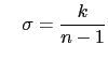
It is possible to define a simple regular vertical grid by giving zero stretching (ppacr=0).
In that case, the parameters jpk (number of ![]() -levels) and pphmax
(total ocean depth in meters) fully define the grid.
-levels) and pphmax
(total ocean depth in meters) fully define the grid.
For climate-related studies it is often desirable to concentrate the vertical resolution
near the ocean surface. The following function is proposed as a standard for a
![]() -coordinate (with either full or partial steps):
-coordinate (with either full or partial steps):
If the ice shelf cavities are opened (ln_isfcav= true ), the definition of ![]() is the same.
However, definition of
is the same.
However, definition of ![]() at
at ![]() - and
- and ![]() -points is respectively changed to:
-points is respectively changed to:
The most used vertical grid for ORCA2 has ![]() (
(![]() resolution in the
surface (bottom) layers and a depth which varies from 0 at the sea surface to a
minimum of
resolution in the
surface (bottom) layers and a depth which varies from 0 at the sea surface to a
minimum of ![]() . This leads to the following conditions:
. This leads to the following conditions:
With the choice of the stretching ![]() and the number of levels
jpk=
and the number of levels
jpk=![]() , the four coefficients
, the four coefficients ![]() ,
, ![]() ,
, ![]() , and
, and ![]() in
(4.14) have been determined such that (4.15) is
satisfied, through an optimisation procedure using a bisection method. For the first
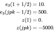
standard ORCA2 vertical grid this led to the following values:
in
(4.14) have been determined such that (4.15) is
satisfied, through an optimisation procedure using a bisection method. For the first
standard ORCA2 vertical grid this led to the following values:
![]() ,
,
![]() , and
, and
![]() . The resulting depths and
scale factors as a function of the model levels are shown in Fig. 4.6 and
given in Table 4.2. Those values correspond to the parameters
ppsur, ppa0, ppa1, ppkth in namcfg namelist.
. The resulting depths and
scale factors as a function of the model levels are shown in Fig. 4.6 and
given in Table 4.2. Those values correspond to the parameters
ppsur, ppa0, ppa1, ppkth in namcfg namelist.
Rather than entering parameters ![]() ,
, ![]() , and
, and ![]() directly, it is
possible to recalculate them. In that case the user sets
ppsur=ppa0=ppa1=999999., in namcfg namelist,
and specifies instead the four following parameters:
directly, it is
possible to recalculate them. In that case the user sets
ppsur=ppa0=ppa1=999999., in namcfg namelist,
and specifies instead the four following parameters:
|
!-----------------------------------------------------------------------
&namdom        !   space and time domain (bathymetry, mesh, timestep)
!-----------------------------------------------------------------------
   nn_bathy    =    1      !  compute (=0) or read (=1) the bathymetry file
   rn_bathy    =    0.     !  value of the bathymetry. if (=0) bottom flat at jpkm1
   nn_closea   =    0      !  remove (=0) or keep (=1) closed seas and lakes (ORCA)
   nn_msh      =    1      !  create (=1) a mesh file or not (=0)
   rn_hmin     =   -3.     !  min depth of the ocean (>0) or min number of ocean level (<0)
   rn_e3zps_min=   20.     !  partial step thickness is set larger than the minimum of
   rn_e3zps_rat=    0.1    !  rn_e3zps_min and rn_e3zps_rat*e3t, with 0<rn_e3zps_rat<1
                           !
   rn_rdt      = 5760.     !  time step for the dynamics (and tracer if nn_acc=0)
   rn_atfp     =    0.1    !  asselin time filter parameter
   nn_acc      =    0      !  acceleration of convergence : =1      used, rdt < rdttra(k)
                                 !                          =0, not used, rdt = rdttra
   rn_rdtmin   = 28800.          !  minimum time step on tracers (used if nn_acc=1)
   rn_rdtmax   = 28800.          !  maximum time step on tracers (used if nn_acc=1)
   rn_rdth     =  800.           !  depth variation of tracer time step  (used if nn_acc=1)
   ln_crs      = .false.      !  Logical switch for coarsening module
   jphgr_msh   =       0               !  type of horizontal mesh
                                       !  = 0 curvilinear coordinate on the sphere read in coordinate.nc
                                       !  = 1 geographical mesh on the sphere with regular grid-spacing
                                       !  = 2 f-plane with regular grid-spacing
                                       !  = 3 beta-plane with regular grid-spacing
                                       !  = 4 Mercator grid with T/U point at the equator
   ppglam0     =       0.0             !  longitude of first raw and column T-point (jphgr_msh = 1)
   ppgphi0     =     -35.0             ! latitude  of first raw and column T-point (jphgr_msh = 1)
   ppe1_deg    =       1.0             !  zonal      grid-spacing (degrees)
   ppe2_deg    =       0.5             !  meridional grid-spacing (degrees)
   ppe1_m      =    5000.0             !  zonal      grid-spacing (degrees)
   ppe2_m      =    5000.0             !  meridional grid-spacing (degrees)
   ppsur       =    -4762.96143546300  !  ORCA r4, r2 and r05 coefficients
   ppa0        =      255.58049070440  ! (default coefficients)
   ppa1        =      245.58132232490  !
   ppkth       =       21.43336197938  !
   ppacr       =        3.0            !
   ppdzmin     =       10.             !  Minimum vertical spacing
   pphmax      =     5000.             !  Maximum depth
   ldbletanh   =    .TRUE.             !  Use/do not use double tanf function for vertical coordinates
   ppa2        =      100.760928500000 !  Double tanh function parameters
   ppkth2      =       48.029893720000 !
   ppacr2      =       13.000000000000 !
/
In ![]() -coordinate partial step, the depths of the model levels are defined by the
reference analytical function
-coordinate partial step, the depths of the model levels are defined by the
reference analytical function ![]() as described in the previous
section, except in the bottom layer. The thickness of the bottom layer is
allowed to vary as a function of geographical location
as described in the previous
section, except in the bottom layer. The thickness of the bottom layer is
allowed to vary as a function of geographical location
![]() to allow a
better representation of the bathymetry, especially in the case of small
slopes (where the bathymetry varies by less than one level thickness from
one grid point to the next). The reference layer thicknesses
to allow a
better representation of the bathymetry, especially in the case of small
slopes (where the bathymetry varies by less than one level thickness from
one grid point to the next). The reference layer thicknesses ![]() have been
defined in the absence of bathymetry. With partial steps, layers from 1 to
jpk-2 can have a thickness smaller than
have been
defined in the absence of bathymetry. With partial steps, layers from 1 to
jpk-2 can have a thickness smaller than
![]() . The model deepest layer (jpk-1)
is allowed to have either a smaller or larger thickness than
. The model deepest layer (jpk-1)
is allowed to have either a smaller or larger thickness than
![]() : the
maximum thickness allowed is
: the
maximum thickness allowed is
![]() . This has to be kept in mind when
specifying values in namdom namelist, as the maximum depth pphmax
in partial steps: for example, with
pphmax
. This has to be kept in mind when
specifying values in namdom namelist, as the maximum depth pphmax
in partial steps: for example, with
pphmax![]() for the DRAKKAR 45 layer grid, the maximum ocean depth
allowed is actually
for the DRAKKAR 45 layer grid, the maximum ocean depth
allowed is actually ![]() (the default thickness
(the default thickness
![]() being
being ![]() ).
Two variables in the namdom namelist are used to define the partial step
vertical grid. The mimimum water thickness (in meters) allowed for a cell
partially filled with bathymetry at level jk is the minimum of rn_e3zps_min
(thickness in meters, usually
).
Two variables in the namdom namelist are used to define the partial step
vertical grid. The mimimum water thickness (in meters) allowed for a cell
partially filled with bathymetry at level jk is the minimum of rn_e3zps_min
(thickness in meters, usually ![]() ) or
) or
![]() (a fraction,
usually 10%, of the default thickness
(a fraction,
usually 10%, of the default thickness
![]() ).
).
!-----------------------------------------------------------------------
&namzgr_sco    !   s-coordinate or hybrid z-s-coordinate
!-----------------------------------------------------------------------
   ln_s_sh94   = .true.    !  Song & Haidvogel 1994 hybrid S-sigma   (T)|
   ln_s_sf12   = .false.   !  Siddorn & Furner 2012 hybrid S-z-sigma (T)| if both are false the NEMO tanh stretching is applied
   ln_sigcrit  = .false.   !  use sigma coordinates below critical depth (T) or Z coordinates (F) for Siddorn & Furner stretch
                           !  stretching coefficients for all functions
   rn_sbot_min =   10.0    !  minimum depth of s-bottom surface (>0) (m)
   rn_sbot_max = 7000.0    !  maximum depth of s-bottom surface (= ocean depth) (>0) (m)
   rn_hc       =  150.0    !  critical depth for transition to stretched coordinates
                        !!!!!!!  Envelop bathymetry
   rn_rmax     =    0.3    !  maximum cut-off r-value allowed (0<r_max<1)
                        !!!!!!!  SH94 stretching coefficients  (ln_s_sh94 = .true.)
   rn_theta    =    6.0    !  surface control parameter (0<=theta<=20)
   rn_bb       =    0.8    !  stretching with SH94 s-sigma
                        !!!!!!!  SF12 stretching coefficient  (ln_s_sf12 = .true.)
   rn_alpha    =    4.4    !  stretching with SF12 s-sigma
   rn_efold    =    0.0    !  efold length scale for transition to stretched coord
   rn_zs       =    1.0    !  depth of surface grid box
                           !  bottom cell depth (Zb) is a linear function of water depth Zb = H*a + b
   rn_zb_a     =    0.024  !  bathymetry scaling factor for calculating Zb
   rn_zb_b     =   -0.2    !  offset for calculating Zb
                        !!!!!!!! Other stretching (not SH94 or SF12) [also uses rn_theta above]
   rn_thetb    =    1.0    !  bottom control parameter  (0<=thetb<= 1)
/
where ![]() is the depth of the last
is the depth of the last ![]() -level (
-level (![]() ) defined at the
) defined at the ![]() -point
location in the horizontal and
-point
location in the horizontal and ![]() is a function which varies from 0 at the sea
surface to
is a function which varies from 0 at the sea
surface to ![]() at the ocean bottom. The depth field
at the ocean bottom. The depth field ![]() is not necessary the ocean
depth, since a mixed step-like and bottom-following representation of the
topography can be used (Fig. 4.5d-e) or an envelop bathymetry can be defined (Fig. 4.5f).
The namelist parameter rn_rmax determines the slope at which the terrain-following coordinate intersects the sea bed and becomes a pseudo z-coordinate. The coordinate can also be hybridised by specifying rn_sbot_min and rn_sbot_max as the minimum and maximum depths at which the terrain-following vertical coordinate is calculated.
is not necessary the ocean
depth, since a mixed step-like and bottom-following representation of the
topography can be used (Fig. 4.5d-e) or an envelop bathymetry can be defined (Fig. 4.5f).
The namelist parameter rn_rmax determines the slope at which the terrain-following coordinate intersects the sea bed and becomes a pseudo z-coordinate. The coordinate can also be hybridised by specifying rn_sbot_min and rn_sbot_max as the minimum and maximum depths at which the terrain-following vertical coordinate is calculated.
Options for stretching the coordinate are provided as examples, but care must be taken to ensure that the vertical stretch used is appropriate for the application.
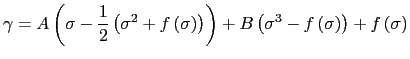
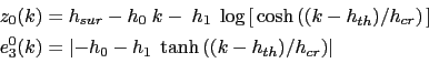
The original default NEMO s-coordinate stretching is available if neither of the other options are specified as true (ln_sco_SH94 = false and ln_sco_SF12 = false.) This uses a depth independent ![]() function for the stretching [Madec et al., 1996]:
function for the stretching [Madec et al., 1996]:
where ![]() is the depth at which the s-coordinate stretching starts and allows a z-coordinate to placed on top of the stretched coordinate, and z is the depth (negative down from the asea surface).
is the depth at which the s-coordinate stretching starts and allows a z-coordinate to placed on top of the stretched coordinate, and z is the depth (negative down from the asea surface).
A stretching function, modified from the commonly used Song and Haidvogel [1994] stretching (ln_sco_SH94 = true), is also available and is more commonly used for shelf seas modelling:
![\includegraphics[width=1.0\textwidth]{Fig_sco_function}](img461.png)
|
where ![]() is the critical depth (rn_hc) at which the coordinate transitions from pure
is the critical depth (rn_hc) at which the coordinate transitions from pure ![]() to the stretched coordinate, and
to the stretched coordinate, and ![]() (rn_theta) and
(rn_theta) and ![]() (rn_bb) are the surface and
bottom control parameters such that
(rn_bb) are the surface and
bottom control parameters such that
![]() , and
, and
![]() .
. ![]() has been designed to allow surface and/or bottom
increase of the vertical resolution (Fig. 4.7).
has been designed to allow surface and/or bottom
increase of the vertical resolution (Fig. 4.7).
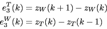
Another example has been provided at version 3.5 (ln_sco_SF12) that allows a fixed surface resolution in an analytical terrain-following stretching Siddorn and Furner [2012]. In this case the a stretching function ![]() is defined such that:
is defined such that:
The function is defined with respect to ![]() , the unstretched terrain-following coordinate:
, the unstretched terrain-following coordinate:
Where:
This gives an analytical stretching of ![]() that is solvable in
that is solvable in ![]() and
and ![]() as a function of the user prescribed stretching parameter
as a function of the user prescribed stretching parameter ![]() (rn_alpha) that stretches towards the surface (
(rn_alpha) that stretches towards the surface (
![]() ) or the bottom (
) or the bottom (
![]() ) and user prescribed surface (rn_zs) and bottom depths. The bottom cell depth in this example is given as a function of water depth:
) and user prescribed surface (rn_zs) and bottom depths. The bottom cell depth in this example is given as a function of water depth:
where the namelist parameters rn_zb_a and rn_zb_b are ![]() and
and ![]() respectively.
respectively.
![\includegraphics[width=1.0\textwidth]{FIG_DOM_compare_coordinates_surface}](img477.png) |
This gives a smooth analytical stretching in computational space that is constrained to given specified surface and bottom grid cell thicknesses in real space. This is not to be confused with the hybrid schemes that superimpose geopotential coordinates on terrain following coordinates thus creating a non-analytical vertical coordinate that therefore may suffer from large gradients in the vertical resolutions. This stretching is less straightforward to implement than the Song and Haidvogel [1994] stretching, but has the advantage of resolving diurnal processes in deep water and has generally flatter slopes.
As with the Song and Haidvogel [1994] stretching the stretch is only applied at depths greater than the critical depth ![]() . In this example two options are available in depths shallower than
. In this example two options are available in depths shallower than ![]() , with pure sigma being applied if the ln_sigcrit is true and pure z-coordinates if it is false (the z-coordinate being equal to the depths of the stretched coordinate at
, with pure sigma being applied if the ln_sigcrit is true and pure z-coordinates if it is false (the z-coordinate being equal to the depths of the stretched coordinate at ![]() .
.
Minimising the horizontal slope of the vertical coordinate is important in terrain-following systems as large slopes lead to hydrostatic consistency. A hydrostatic consistency parameter diagnostic following Haney [1991] has been implemented, and is output as part of the model mesh file at the start of the run.
This option is described in the Report by Levier et al. (2007), available on the NEMO web site.
Whatever the vertical coordinate used, the model offers the possibility of
representing the bottom topography with steps that follow the face of the
model cells (step like topography) [Madec et al., 1996]. The distribution of
the steps in the horizontal is defined in a 2D integer array, mbathy, which
gives the number of ocean levels (![]() those that are not masked) at each
those that are not masked) at each
![]() -point. mbathy is computed from the meter bathymetry using the definiton of
gdept as the number of
-point. mbathy is computed from the meter bathymetry using the definiton of
gdept as the number of ![]() -points which gdept
-points which gdept ![]() bathy.
bathy.
Modifications of the model bathymetry are performed in the bat_ctl
routine (see domzgr.F90 module) after mbathy is computed. Isolated grid points
that do not communicate with another ocean point at the same level are eliminated.
As for the representation of bathymetry, a 2D integer array, misfdep, is created.
misfdep defines the level of the first wet ![]() -point. All the cells between
-point. All the cells between ![]() and
and
![]() are masked.
By default, misfdep(:,:)=1 and no cells are masked.
are masked.
By default, misfdep(:,:)=1 and no cells are masked.
In case of ice shelf cavities (ln_isfcav = true), modifications of the model bathymetry and ice shelf draft in
the cavities are performed through the zgr_isf routine. The compatibility between ice shelf draft and bathymetry is checked:
if only one cell on the water column is opened at ![]() -,
-, ![]() - or
- or  -points, the bathymetry or the ice shelf draft is dug to have a 2-level water column
(i.e. two unmasked levels). If the incompatibility is too strong (i.e. need to dig more than one cell), the entire water column is masked.
-points, the bathymetry or the ice shelf draft is dug to have a 2-level water column
(i.e. two unmasked levels). If the incompatibility is too strong (i.e. need to dig more than one cell), the entire water column is masked.
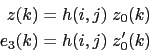
From the mbathy array, the mask fields are defined as follows:
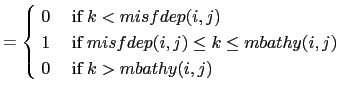 |
||
Note, wmask is now defined. It allows, in case of ice shelves, to deal with the top boundary (ice shelf/ocean interface) exactly in the same way as for the bottom boundary.
The specification of closed lateral boundaries requires that at least the first and last rows and columns of the mbathy array are set to zero. In the particular case of an east-west cyclical boundary condition, mbathy has its last column equal to the second one and its first column equal to the last but one (and so too the mask arrays) (see § 8.2).
Gurvan Madec and the NEMO Team
NEMO European Consortium2017-02-17
![\includegraphics[width=1.0\textwidth]{Fig_z_zps_s_sps}](img408.png)
 and
and ![$\displaystyle C\left(s\right) = \left(1 - b \right)\frac{ \sinh\left( \theta s\...
...t] - \tanh\left(\frac{\theta}{2}\right)}{ 2\tanh\left (\frac{\theta}{2}\right)}$](img460.png)