Next: Tracer Equation Up: Curvilinear Coordinate Equations Previous: Continuity Equation in coordinates Contents Index
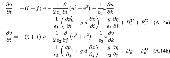
Here we only consider the first component of the momentum equation, the generalization to the second one being straightforward.
![]()
![]() Total derivative in vector invariant form
Total derivative in vector invariant form
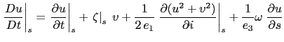
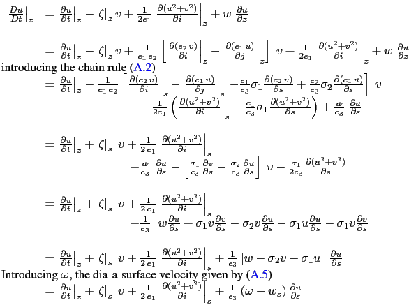
Let us consider (2.13), the first component of the momentum
equation in the vector invariant form. Its total ![]() coordinate time derivative,
coordinate time derivative,
![]() can be transformed as follows in order to obtain
its expression in the curvilinear
can be transformed as follows in order to obtain
its expression in the curvilinear ![]() coordinate system:
coordinate system:
 |
![]()
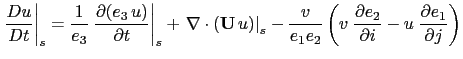
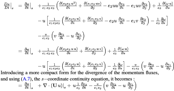
![]() Total derivative in flux form
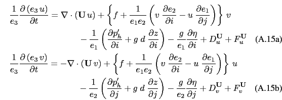
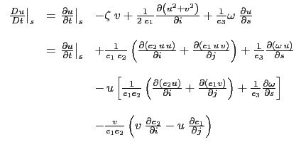
Total derivative in flux form
Let us start from the total time derivative in the curvilinear ![]() coordinate system
we have just establish. Following the procedure used to establish (2.11),
it can be transformed into :
coordinate system
we have just establish. Following the procedure used to establish (2.11),
it can be transformed into :
 |
 |
![]()
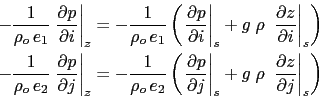
![]() horizontal pressure gradient
horizontal pressure gradient
The horizontal pressure gradient term can be transformed as follows:
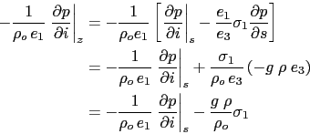 |
An additional term appears in (A.14) which accounts for the
tilt of ![]() surfaces with respect to geopotential
surfaces with respect to geopotential ![]() surfaces.
surfaces.
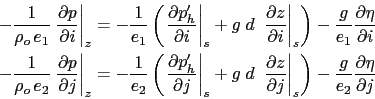
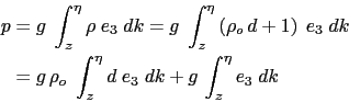
As in ![]() -coordinate, the horizontal pressure gradient can be split in two parts
following Marsaleix et al. [2008]. Let defined a density anomaly,
-coordinate, the horizontal pressure gradient can be split in two parts
following Marsaleix et al. [2008]. Let defined a density anomaly, ![]() , by
, by
![]() ,
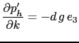
and a hydrostatic pressure anomaly,
,
and a hydrostatic pressure anomaly, ![]() , by
, by
![]() .
The pressure is then given by:
.
The pressure is then given by:
 |
 |
Substituing (A.13) in (A.14) and using the definition of the density anomaly it comes the expression in two parts:
![]()
![]() The other terms of the momentum equation
The other terms of the momentum equation
The coriolis and forcing terms as well as the the vertical physics remain unchanged as they involve neither time nor space derivatives. The form of the lateral physics is discussed in appendix B.
![]()
![]() Full momentum equation
Full momentum equation
To sum up, in a curvilinear ![]() -coordinate system, the vector invariant momentum equation
solved by the model has the same mathematical expression as the one in a curvilinear
-coordinate system, the vector invariant momentum equation
solved by the model has the same mathematical expression as the one in a curvilinear
![]() coordinate, except for the pressure gradient term :
coordinate, except for the pressure gradient term :
It is important to realize that the change in coordinate system has only concerned
the position on the vertical. It has not affected (i,j,k), the
orthogonal curvilinear set of unit vectors. (![]() ,
, ) are always horizontal velocities
so that their evolution is driven by horizontal forces, in particular
the pressure gradient. By contrast,
) are always horizontal velocities
so that their evolution is driven by horizontal forces, in particular
the pressure gradient. By contrast, ![]() is not
is not ![]() , the third component of the velocity,
but the dia-surface velocity component,
, the third component of the velocity,
but the dia-surface velocity component, ![]() the volume flux across the moving
the volume flux across the moving
![]() -surfaces per unit horizontal area.
-surfaces per unit horizontal area.
Gurvan Madec and the NEMO Team
NEMO European Consortium2017-02-17