Subsections
Primitive Equations
Vector Invariant Formulation
The ocean is a fluid that can be described to a good approximation by the primitive
equations,  the Navier-Stokes equations along with a nonlinear equation of
state which couples the two active tracers (temperature and salinity) to the fluid
velocity, plus the following additional assumptions made from scale considerations:
the Navier-Stokes equations along with a nonlinear equation of
state which couples the two active tracers (temperature and salinity) to the fluid
velocity, plus the following additional assumptions made from scale considerations:
(1) spherical earth approximation: the geopotential surfaces are assumed to
be spheres so that gravity (local vertical) is parallel to the earth's radius
(2) thin-shell approximation: the ocean depth is neglected compared to the earth's radius
(3) turbulent closure hypothesis: the turbulent fluxes (which represent the effect
of small scale processes on the large-scale) are expressed in terms of large-scale features
(4) Boussinesq hypothesis: density variations are neglected except in their
contribution to the buoyancy force
(5) Hydrostatic hypothesis: the vertical momentum equation is reduced to a
balance between the vertical pressure gradient and the buoyancy force (this removes
convective processes from the initial Navier-Stokes equations and so convective processes
must be parameterized instead)
(6) Incompressibility hypothesis: the three dimensional divergence of the velocity
vector is assumed to be zero.
Because the gravitational force is so dominant in the equations of large-scale motions,
it is useful to choose an orthogonal set of unit vectors (i,j,k) linked
to the earth such that k is the local upward vector and (i,j) are two
vectors orthogonal to k, tangent to the geopotential surfaces. Let us define
the following variables: U the vector velocity,
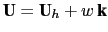 (the subscript
  denotes the local horizontal vector, over the (i,j) plane),
 the potential temperature,
  the salinity,
  the in situ density.
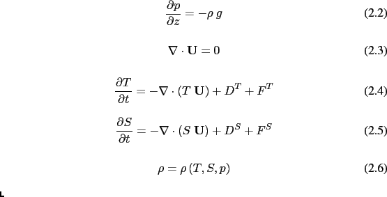
The vector invariant form of the primitive equations in the (i,j,k)
vector system provides the following six equations (namely the momentum balance, the
hydrostatic equilibrium, the incompressibility equation, the heat and salt conservation
equations and an equation of state):
the in situ density.
The vector invariant form of the primitive equations in the (i,j,k)
vector system provides the following six equations (namely the momentum balance, the
hydrostatic equilibrium, the incompressibility equation, the heat and salt conservation
equations and an equation of state):
where  is the generalised derivative vector operator in
 directions,
 is the time,
  is the vertical coordinate, is the in situ density given by
the equation of state (2.1f),
is the vertical coordinate, is the in situ density given by
the equation of state (2.1f),  is a reference density,
  the pressure,
 is the Coriolis acceleration (where
  is the Earth's
angular velocity vector), and
is the Earth's
angular velocity vector), and  is the gravitational acceleration.
 ,
,  and
and  are the parameterisations of small-scale
physics for momentum, temperature and salinity, and
are the parameterisations of small-scale
physics for momentum, temperature and salinity, and
 ,
,  and
and  surface forcing terms. Their nature and formulation are discussed in
§2.5 and page §2.1.2.
surface forcing terms. Their nature and formulation are discussed in
§2.5 and page §2.1.2.
.
Boundary Conditions
An ocean is bounded by complex coastlines, bottom topography at its base and an air-sea
or ice-sea interface at its top. These boundaries can be defined by two surfaces,  and
and
 , where
  is the depth of the ocean bottom and
  is the height
of the sea surface. Both and are usually referenced to a given surface,
is the height
of the sea surface. Both and are usually referenced to a given surface,  ,
chosen as a mean sea surface (Fig. 2.1). Through these two boundaries,
the ocean can exchange fluxes of heat, fresh water, salt, and momentum with the solid earth,
the continental margins, the sea ice and the atmosphere. However, some of these fluxes are
so weak that even on climatic time scales of thousands of years they can be neglected.
In the following, we briefly review the fluxes exchanged at the interfaces between the ocean
and the other components of the earth system.
,
chosen as a mean sea surface (Fig. 2.1). Through these two boundaries,
the ocean can exchange fluxes of heat, fresh water, salt, and momentum with the solid earth,
the continental margins, the sea ice and the atmosphere. However, some of these fluxes are
so weak that even on climatic time scales of thousands of years they can be neglected.
In the following, we briefly review the fluxes exchanged at the interfaces between the ocean
and the other components of the earth system.
Figure 2.1:
The ocean is bounded by two surfaces, and
 , where
is the depth of the sea floor and the height of the sea surface.
Both and are referenced to .
, where
is the depth of the sea floor and the height of the sea surface.
Both and are referenced to .
|
|
- Land - ocean interface:
- the major flux between continental margins and the ocean is
a mass exchange of fresh water through river runoff. Such an exchange modifies the sea
surface salinity especially in the vicinity of major river mouths. It can be neglected for short
range integrations but has to be taken into account for long term integrations as it influences
the characteristics of water masses formed (especially at high latitudes). It is required in order
to close the water cycle of the climate system. It is usually specified as a fresh water flux at
the air-sea interface in the vicinity of river mouths.
- Solid earth - ocean interface:
- heat and salt fluxes through the sea floor are small,
except in special areas of little extent. They are usually neglected in the model
2.1.
The boundary condition is thus set to no flux of heat and salt across solid boundaries.
For momentum, the situation is different. There is no flow across solid boundaries,
the velocity normal to the ocean bottom and coastlines is zero (in other words,
the bottom velocity is parallel to solid boundaries). This kinematic boundary condition
can be expressed as:
 |
(2.2) |
In addition, the ocean exchanges momentum with the earth through frictional processes.
Such momentum transfer occurs at small scales in a boundary layer. It must be parameterized
in terms of turbulent fluxes using bottom and/or lateral boundary conditions. Its specification
depends on the nature of the physical parameterisation used for
in (2.1a). It is discussed in §2.5.1, page ![[*]](crossref.png) .
.
- Atmosphere - ocean interface:
- the kinematic surface condition plus the mass flux
of fresh water PE (the precipitation minus evaporation budget) leads to:
 |
(2.3) |
The dynamic boundary condition, neglecting the surface tension (which removes capillary
waves from the system) leads to the continuity of pressure across the interface  .
The atmosphere and ocean also exchange horizontal momentum (wind stress), and heat.
.
The atmosphere and ocean also exchange horizontal momentum (wind stress), and heat.
- Sea ice - ocean interface:
- the ocean and sea ice exchange heat, salt, fresh water
and momentum. The sea surface temperature is constrained to be at the freezing point
at the interface. Sea ice salinity is very low (
 ) compared to those of the
ocean (
) compared to those of the
ocean (
 ). The cycle of freezing/melting is associated with fresh water and
salt fluxes that cannot be neglected.
). The cycle of freezing/melting is associated with fresh water and
salt fluxes that cannot be neglected.
Footnotes
- ... model2.1
- In fact, it has been shown that the heat flux associated with the solid Earth cooling
(the geothermal heating) is not negligible for the thermohaline circulation of the world
ocean (see 5.4.3).
Gurvan Madec and the NEMO Team
NEMO European Consortium2017-02-17
![\includegraphics[width=0.90\textwidth]{Fig_I_ocean_bc}](img126.png)