The Horizontal Pressure Gradient

Pressure Formulation

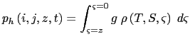
The total pressure at a given depth $z$ is composed of a surface pressure $p_s$ at a reference geopotential surface ($z=0$) and a hydrostatic pressure $p_h$ such that: $p(i,j,k,t)=p_s(i,j,t)+p_h(i,j,k,t)$. The latter is computed by integrating (2.1b), assuming that pressure in decibars can be approximated by depth in meters in (2.1f). The hydrostatic pressure is then given by:

$$p_h \left( {i,j,z,t} \right) = \int_{\varsigma =z}^{\varsigma =0} {g\;\rho \left( {T,S,\varsigma} \right)\;d\varsigma }$$ (2.4)

Two strategies can be considered for the surface pressure term: $(a)$ introduce of a new variable $\eta$, the free-surface elevation, for which a prognostic equation can be established and solved; $(b)$ assume that the ocean surface is a rigid lid, on which the pressure (or its horizontal gradient) can be diagnosed. When the former strategy is used, one solution of the free-surface elevation consists of the excitation of external gravity waves. The flow is barotropic and the surface moves up and down with gravity as the restoring force. The phase speed of such waves is high (some hundreds of metres per second) so that the time step would have to be very short if they were present in the model. The latter strategy filters out these waves since the rigid lid approximation implies $\eta=0$, $i.e.$ the sea surface is the surface $z=0$. This well known approximation increases the surface wave speed to infinity and modifies certain other longwave dynamics ($e.g.$ barotropic Rossby or planetary waves). The rigid-lid hypothesis is an obsolescent feature in modern OGCMs. It has been available until the release 3.1 of NEMO, and it has been removed in release 3.2 and followings. Only the free surface formulation is now described in the this document (see the next sub-section).

Free Surface Formulation

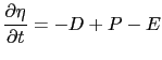
In the free surface formulation, a variable $\eta$, the sea-surface height, is introduced which describes the shape of the air-sea interface. This variable is solution of a prognostic equation which is established by forming the vertical average of the kinematic surface condition (2.2):

$$\frac{\partial \eta }{\partial t}=-D+P-E D=\nabla \cdot \left[ {\left( {H+\eta } \right) \; {\rm {\bf\overline{U}}}_h } \right]$$ (2.5)

and using (2.1b) the surface pressure is given by: $p_s = \rho g \eta$.

Allowing the air-sea interface to move introduces the external gravity waves (EGWs) as a class of solution of the primitive equations. These waves are barotropic because of hydrostatic assumption, and their phase speed is quite high. Their time scale is short with respect to the other processes described by the primitive equations.

Two choices can be made regarding the implementation of the free surface in the model, depending on the physical processes of interest.

$\bullet$ If one is interested in EGWs, in particular the tides and their interaction with the baroclinic structure of the ocean (internal waves) possibly in shallow seas, then a non linear free surface is the most appropriate. This means that no approximation is made in (2.5) and that the variation of the ocean volume is fully taken into account. Note that in order to study the fast time scales associated with EGWs it is necessary to minimize time filtering effects (use an explicit time scheme with very small time step, or a split-explicit scheme with reasonably small time step, see §6.5.1 or §6.5.2.

$\bullet$ If one is not interested in EGW but rather sees them as high frequency noise, it is possible to apply an explicit filter to slow down the fastest waves while not altering the slow barotropic Rossby waves. If further, an approximative conservation of heat and salt contents is sufficient for the problem solved, then it is sufficient to solve a linearized version of (2.5), which still allows to take into account freshwater fluxes applied at the ocean surface [Roullet and Madec, 2000]. Nevertheless, with the linearization, an exact conservation of heat and salt contents is lost.

The filtering of EGWs in models with a free surface is usually a matter of discretisation of the temporal derivatives, using a split-explicit method [Zhang and Endoh, 1992, Killworth et al., 1991] or the implicit scheme [Dukowicz and Smith, 1994] or the addition of a filtering force in the momentum equation [Roullet and Madec, 2000]. With the present release, NEMO offers the choice between an explicit free surface (see §6.5.1) or a split-explicit scheme strongly inspired the one proposed by Shchepetkin and McWilliams [2005] (see §6.5.2).