External Forcing

Surface boundary condition (trasbc.F90)

The surface boundary condition for tracers is implemented in a separate module (trasbc.F90) instead of entering as a boundary condition on the vertical diffusion operator (as in the case of momentum). This has been found to enhance readability of the code. The two formulations are completely equivalent; the forcing terms in trasbc are the surface fluxes divided by the thickness of the top model layer.

Due to interactions and mass exchange of water ($F_{mass}$) with other Earth system components ($i.e.$ atmosphere, sea-ice, land), the change in the heat and salt content of the surface layer of the ocean is due both to the heat and salt fluxes crossing the sea surface (not linked with $F_{mass}$) and to the heat and salt content of the mass exchange. They are both included directly in $Q_{ns}$, the surface heat flux, and $F_{salt}$, the surface salt flux (see §7 for further details). By doing this, the forcing formulation is the same for any tracer (including temperature and salinity).

The surface module (sbcmod.F90, see §7) provides the following forcing fields (used on tracers):

$\bullet$ $Q_{ns}$, the non-solar part of the net surface heat flux that crosses the sea surface (i.e. the difference between the total surface heat flux and the fraction of the short wave flux that penetrates into the water column, see §5.4.2) plus the heat content associated with of the mass exchange with the atmosphere and lands.

$\bullet$ $\textit{sfx}$, the salt flux resulting from ice-ocean mass exchange (freezing, melting, ridging...)

$\bullet$ emp, the mass flux exchanged with the atmosphere (evaporation minus precipitation) and possibly with the sea-ice and ice-shelves.

$\bullet$ rnf, the mass flux associated with runoff (see §7.9 for further detail of how it acts on temperature and salinity tendencies)

$\bullet$ fwfisf, the mass flux associated with ice shelf melt, (see §7.10 for further details on how the ice shelf melt is computed and applied).

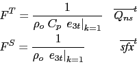
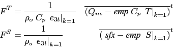
In the non-linear free surface case (key_ vvl is defined), the surface boundary condition on temperature and salinity is applied as follows:

$$\begin{aligned}&F^T = \frac{ 1 }{\rho _o \;C_p \left. e_{3t} ... ...ght\vert _{k=1} } &\overline{ \textit{sfx} }^t & \end{aligned}$$

where $\overline{x }^t$ means that $x$ is averaged over two consecutive time steps ($t-\rdt/2$ and $t+\rdt/2$). Such time averaging prevents the divergence of odd and even time step (see §3).

In the linear free surface case (key_ vvl is not defined), an additional term has to be added on both temperature and salinity. On temperature, this term remove the heat content associated with mass exchange that has been added to $Q_{ns}$. On salinity, this term mimics the concentration/dilution effect that would have resulted from a change in the volume of the first level. The resulting surface boundary condition is applied as follows:

$$\begin{aligned}&F^T = \frac{ 1 }{\rho _o \;C_p \left. e_{3t} ... ...emp} \;\left. S \right\vert _{k=1} \right) }^t & \end{aligned}$$

Note that an exact conservation of heat and salt content is only achieved with non-linear free surface. In the linear free surface case, there is a small imbalance. The imbalance is larger than the imbalance associated with the Asselin time filter [Leclair and Madec, 2009]. This is the reason why the modified filter is not applied in the linear free surface case (see §3).

Solar Radiation Penetration (traqsr.F90)

!-----------------------------------------------------------------------
&namtra_qsr    !   penetrative solar radiation
!-----------------------------------------------------------------------
!              !  file name  ! frequency (hours) ! variable  ! time interp. !  clim  ! 'yearly'/ ! weights  ! rotation ! land/sea mask !
!              !             !  (if <0  months)  !   name    !   (logical)  !  (T/F) ! 'monthly' ! filename ! pairing  ! filename      !
   sn_chl      ='chlorophyll',        -1         , 'CHLA'    ,   .true.     , .true. , 'yearly'  , ''       , ''       , ''

   cn_dir      = './'      !  root directory for the location of the runoff files
   ln_traqsr   = .true.    !  Light penetration (T) or not (F)
   ln_qsr_rgb  = .true.    !  RGB (Red-Green-Blue) light penetration
   ln_qsr_2bd  = .false.   !  2 bands              light penetration
   ln_qsr_bio  = .false.   !  bio-model light penetration
   nn_chldta   =      1    !  RGB : 2D Chl data (=1), 3D Chl data (=2) or cst value (=0)
   rn_abs      =   0.58    !  RGB & 2 bands: fraction of light (rn_si1)
   rn_si0      =   0.35    !  RGB & 2 bands: shortess depth of extinction
   rn_si1      =   23.0    !  2 bands: longest depth of extinction
   ln_qsr_ice  = .true.    !  light penetration for ice-model LIM3
/

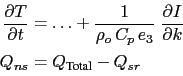
Options are defined through the namtra_qsr namelist variables. When the penetrative solar radiation option is used (ln_flxqsr=true), the solar radiation penetrates the top few tens of meters of the ocean. If it is not used (ln_flxqsr=false) all the heat flux is absorbed in the first ocean level. Thus, in the former case a term is added to the time evolution equation of temperature (2.1d) and the surface boundary condition is modified to take into account only the non-penetrative part of the surface heat flux:

$$\begin{split}\frac{\partial T}{\partial t} &= {\ldots} + \fra... ...I}{\partial k} Q_{ns} &= Q_\text{Total} - Q_{sr} \end{split}$$ (5.13)

where $Q_{sr}$ is the penetrative part of the surface heat flux ($i.e.$ the shortwave radiation) and $I$ is the downward irradiance ( $\left. I \right\vert _{z=\eta}=Q_{sr}$). The additional term in (5.13) is discretized as follows:

$$\frac{1}{\rho_o C_p e_3} \; \frac{\partial I}{\partial k} \equiv \frac{1}{\rho_o C_p e_{3t}} \delta_k \left[ I_w \right]$$ (5.14)

The shortwave radiation, $Q_{sr}$, consists of energy distributed across a wide spectral range. The ocean is strongly absorbing for wavelengths longer than 700 nm and these wavelengths contribute to heating the upper few tens of centimetres. The fraction of $Q_{sr}$ that resides in these almost non-penetrative wavebands, $R$, is $\sim 58\%$ (specified through namelist parameter rn_abs). It is assumed to penetrate the ocean with a decreasing exponential profile, with an e-folding depth scale, $\xi_0$, of a few tens of centimetres (typically $\xi_0=0.35 m$ set as rn_si0 in the namtra_qsr namelist). For shorter wavelengths (400-700 nm), the ocean is more transparent, and solar energy propagates to larger depths where it contributes to local heating. The way this second part of the solar energy penetrates into the ocean depends on which formulation is chosen. In the simple 2-waveband light penetration scheme (ln_qsr_2bd=true) a chlorophyll-independent monochromatic formulation is chosen for the shorter wavelengths, leading to the following expression [Paulson and Simpson, 1977]:

$$I(z) = Q_{sr} \left[Re^{-z / \xi_0} + \left( 1-R\right) e^{-z / \xi_1} \right]$$ (5.15)

where $\xi_1$ is the second extinction length scale associated with the shorter wavelengths. It is usually chosen to be 23 m by setting the rn_si0 namelist parameter. The set of default values ($\xi_0$, $\xi_1$, $R$) corresponds to a Type I water in Jerlov's (1968) classification (oligotrophic waters).

Such assumptions have been shown to provide a very crude and simplistic representation of observed light penetration profiles (Morel [1988], see also Fig.5.2). Light absorption in the ocean depends on particle concentration and is spectrally selective. Morel [1988] has shown that an accurate representation of light penetration can be provided by a 61 waveband formulation. Unfortunately, such a model is very computationally expensive. Thus, Lengaigne et al. [2007] have constructed a simplified version of this formulation in which visible light is split into three wavebands: blue (400-500 nm), green (500-600 nm) and red (600-700nm). For each wave-band, the chlorophyll-dependent attenuation coefficient is fitted to the coefficients computed from the full spectral model of Morel [1988] (as modified by Morel and Maritorena [2001]), assuming the same power-law relationship. As shown in Fig.5.2, this formulation, called RGB (Red-Green-Blue), reproduces quite closely the light penetration profiles predicted by the full spectal model, but with much greater computational efficiency. The 2-bands formulation does not reproduce the full model very well.

The RGB formulation is used when ln_qsr_rgb=true. The RGB attenuation coefficients ($i.e.$ the inverses of the extinction length scales) are tabulated over 61 nonuniform chlorophyll classes ranging from 0.01 to 10 g.Chl/L (see the routine trc_oce_rgb in trc_oce.F90 module). Four types of chlorophyll can be chosen in the RGB formulation:

nn_chdta=0

a constant 0.05 g.Chl/L value everywhere ;

nn_chdta=1

an observed time varying chlorophyll deduced from satellite surface ocean color measurement spread uniformly in the vertical direction ;

nn_chdta=2

same as previous case except that a vertical profile of chlorophyl is used. Following Morel and Berthon [1989], the profile is computed from the local surface chlorophyll value ;

ln_qsr_bio=true

simulated time varying chlorophyll by TOP biogeochemical model. In this case, the RGB formulation is used to calculate both the phytoplankton light limitation in PISCES or LOBSTER and the oceanic heating rate.

The trend in (5.14) associated with the penetration of the solar radiation is added to the temperature trend, and the surface heat flux is modified in routine traqsr.F90.

When the $z$-coordinate is preferred to the $s$-coordinate, the depth of $w-$levels does not significantly vary with location. The level at which the light has been totally absorbed ($i.e.$ it is less than the computer precision) is computed once, and the trend associated with the penetration of the solar radiation is only added down to that level. Finally, note that when the ocean is shallow ($<$ 200 m), part of the solar radiation can reach the ocean floor. In this case, we have chosen that all remaining radiation is absorbed in the last ocean level ($i.e.$ $I$ is masked).

Figure 5.2: Penetration profile of the downward solar irradiance calculated by four models. Two waveband chlorophyll-independent formulation (blue), a chlorophyll-dependent monochromatic formulation (green), 4 waveband RGB formulation (red), 61 waveband Morel (1988) formulation (black) for a chlorophyll concentration of (a) Chl=0.05 mg/m$^3$ and (b) Chl=0.5 mg/m$^3$. From Lengaigne et al. [2007].

Bottom Boundary Condition (trabbc.F90)

!-----------------------------------------------------------------------
&nambbc        !   bottom temperature boundary condition
!-----------------------------------------------------------------------
!              !                              !  (if <0  months)  !  
!              !  file name      ! frequency (hours) ! variable   ! time interp.   !  clim   ! 'yearly'/ ! weights  ! rotation ! land/sea mask !
!              !                 !  (if <0  months)  !   name     !   (logical)    !  (T/F ) ! 'monthly' ! filename ! pairing  ! filename      !
   sn_qgh      ='geothermal_heating.nc',  -12.  , 'heatflow'      ,   .false.      , .true.  , 'yearly'  , ''       , ''       , ''
   !
   cn_dir      = './'      !  root directory for the location of the runoff files
   ln_trabbc   = .true.    !  Apply a geothermal heating at the ocean bottom
   nn_geoflx   =    2      !  geothermal heat flux: = 0 no flux
                           !     = 1 constant flux
                           !     = 2 variable flux (read in geothermal_heating.nc in mW/m2)
   rn_geoflx_cst = 86.4e-3 !  Constant value of geothermal heat flux [W/m2]

/

Figure 5.3: Geothermal Heat flux (in $mW.m^{-2}$) used by Emile-Geay and Madec [2009]. It is inferred from the age of the sea floor and the formulae of Stein and Stein [1992].

Usually it is assumed that there is no exchange of heat or salt through the ocean bottom, $i.e.$ a no flux boundary condition is applied on active tracers at the bottom. This is the default option in NEMO, and it is implemented using the masking technique. However, there is a non-zero heat flux across the seafloor that is associated with solid earth cooling. This flux is weak compared to surface fluxes (a mean global value of $\sim0.1\;W/m^2$ [Stein and Stein, 1992]), but it warms systematically the ocean and acts on the densest water masses. Taking this flux into account in a global ocean model increases the deepest overturning cell ($i.e.$ the one associated with the Antarctic Bottom Water) by a few Sverdrups [Emile-Geay and Madec, 2009].

Options are defined through the namtra_bbc namelist variables. The presence of geothermal heating is controlled by setting the namelist parameter ln_trabbc to true. Then, when nn_geoflx is set to 1, a constant geothermal heating is introduced whose value is given by the nn_geoflx_cst, which is also a namelist parameter. When nn_geoflx is set to 2, a spatially varying geothermal heat flux is introduced which is provided in the geothermal_heating.nc NetCDF file (Fig.5.3) [Emile-Geay and Madec, 2009].