Bottom Boundary Layer (trabbl.F90 - key_ trabbl)

!-----------------------------------------------------------------------
&nambbl        !   bottom boundary layer scheme
!-----------------------------------------------------------------------
   nn_bbl_ldf  =  1      !  diffusive bbl (=1)   or not (=0)
   nn_bbl_adv  =  0      !  advective bbl (=1/2) or not (=0)
   rn_ahtbbl   =  1000.  !  lateral mixing coefficient in the bbl  [m2/s]
   rn_gambbl   =  10.    !  advective bbl coefficient                 [s]
/

Options are defined through the nambbl namelist variables. In a $z$-coordinate configuration, the bottom topography is represented by a series of discrete steps. This is not adequate to represent gravity driven downslope flows. Such flows arise either downstream of sills such as the Strait of Gibraltar or Denmark Strait, where dense water formed in marginal seas flows into a basin filled with less dense water, or along the continental slope when dense water masses are formed on a continental shelf. The amount of entrainment that occurs in these gravity plumes is critical in determining the density and volume flux of the densest waters of the ocean, such as Antarctic Bottom Water, or North Atlantic Deep Water. $z$-coordinate models tend to overestimate the entrainment, because the gravity flow is mixed vertically by convection as it goes ”downstairs” following the step topography, sometimes over a thickness much larger than the thickness of the observed gravity plume. A similar problem occurs in the $s$-coordinate when the thickness of the bottom level varies rapidly downstream of a sill [Willebrand et al., 2001], and the thickness of the plume is not resolved.

The idea of the bottom boundary layer (BBL) parameterisation, first introduced by Beckmann and D"oscher [1997], is to allow a direct communication between two adjacent bottom cells at different levels, whenever the densest water is located above the less dense water. The communication can be by a diffusive flux (diffusive BBL), an advective flux (advective BBL), or both. In the current implementation of the BBL, only the tracers are modified, not the velocities. Furthermore, it only connects ocean bottom cells, and therefore does not include all the improvements introduced by Campin and Goosse [1999].

Diffusive Bottom Boundary layer (nn_bbl_ldf=1)

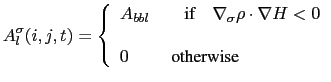
When applying sigma-diffusion (key_ trabbl defined and nn_bbl_ldf set to 1), the diffusive flux between two adjacent cells at the ocean floor is given by

$${\rm {\bf F}}_\sigma=A_l^\sigma \; \nabla_\sigma T$$ (5.16)

with $\nabla_\sigma$ the lateral gradient operator taken between bottom cells, and $A_l^\sigma$ the lateral diffusivity in the BBL. Following Beckmann and D"oscher [1997], the latter is prescribed with a spatial dependence, $i.e.$ in the conditional form

$$A_l^\sigma (i,j,t)=\left\{ {\begin{array}{l} A_{bbl} \quad \quad ... ...cdot \nabla H<0 0\quad \quad \; \mbox{otherwise} \end{array}} \right.$$ (5.17)

where $A_{bbl}$ is the BBL diffusivity coefficient, given by the namelist parameter rn_ahtbbl and usually set to a value much larger than the one used for lateral mixing in the open ocean. The constraint in (5.17) implies that sigma-like diffusion only occurs when the density above the sea floor, at the top of the slope, is larger than in the deeper ocean (see green arrow in Fig.5.4). In practice, this constraint is applied separately in the two horizontal directions, and the density gradient in (5.17) is evaluated with the log gradient formulation:

$$\nabla_\sigma \rho / \rho = \alpha \nabla_\sigma T + \beta \nabla_\sigma S$$ (5.18)

where $\rho$, $\alpha$ and $\beta$ are functions of $\overline{T}^\sigma$, $\overline{S}^\sigma$ and $\overline{H}^\sigma$, the along bottom mean temperature, salinity and depth, respectively.

Advective Bottom Boundary Layer (nn_bbl_adv= 1 or 2)

Figure 5.4: Advective/diffusive Bottom Boundary Layer. The BBL parameterisation is activated when $\rho^i_{kup}$ is larger than $\rho^{i+1}_{kdnw}$. Red arrows indicate the additional overturning circulation due to the advective BBL. The transport of the downslope flow is defined either as the transport of the bottom ocean cell (black arrow), or as a function of the along slope density gradient. The green arrow indicates the diffusive BBL flux directly connecting $kup$ and $kdwn$ ocean bottom cells. connection

When applying an advective BBL (nn_bbl_adv = 1 or 2), an overturning circulation is added which connects two adjacent bottom grid-points only if dense water overlies less dense water on the slope. The density difference causes dense water to move down the slope.

nn_bbl_adv = 1 : the downslope velocity is chosen to be the Eulerian ocean velocity just above the topographic step (see black arrow in Fig.5.4) [Beckmann and D"oscher, 1997]. It is a conditional advection, that is, advection is allowed only if dense water overlies less dense water on the slope ($i.e.$ $\nabla_\sigma \rho \cdot \nabla H<0$) and if the velocity is directed towards greater depth ($i.e.$ $\vect{U} \cdot \nabla H>0$).

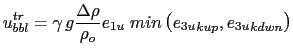
nn_bbl_adv = 2 : the downslope velocity is chosen to be proportional to $\Delta \rho$, the density difference between the higher cell and lower cell densities [Campin and Goosse, 1999]. The advection is allowed only if dense water overlies less dense water on the slope ($i.e.$ $\nabla_\sigma \rho \cdot \nabla H<0$). For example, the resulting transport of the downslope flow, here in the $i$-direction (Fig.5.4), is simply given by the following expression:

$$u^{tr}_{bbl} = \gamma g \frac{\Delta \rho}{\rho_o} e_{1u} \; min \left( {e_{3u}}_{kup},{e_{3u}}_{kdwn} \right)$$ (5.19)

where $\gamma$, expressed in seconds, is the coefficient of proportionality provided as rn_gambbl, a namelist parameter, and kup and kdwn are the vertical index of the higher and lower cells, respectively. The parameter $\gamma$ should take a different value for each bathymetric step, but for simplicity, and because no direct estimation of this parameter is available, a uniform value has been assumed. The possible values for $\gamma$ range between 1 and $10 s$ [Campin and Goosse, 1999].

Scalar properties are advected by this additional transport $( u^{tr}_{bbl}, v^{tr}_{bbl} )$ using the upwind scheme. Such a diffusive advective scheme has been chosen to mimic the entrainment between the downslope plume and the surrounding water at intermediate depths. The entrainment is replaced by the vertical mixing implicit in the advection scheme. 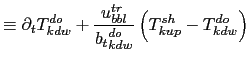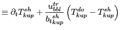Let us consider as an example the case displayed in Fig.5.4 where the density at level $(i,kup)$ is larger than the one at level $(i,kdwn)$. The advective BBL scheme modifies the tracer time tendency of the ocean cells near the topographic step by the downslope flow (5.20), the horizontal (5.21) and the upward (5.22) return flows as follows:

$$\partial_t T^{do}_{kdw} \equiv \partial_t T^{do}_{kdw} + \frac{u^{tr}_{bbl}}{{b_t}^{do}_{kdw}} \left( T^{sh}_{kup} - T^{do}_{kdw} \right)$$ (5.20)

$$\partial_t T^{sh}_{kup} \equiv \partial_t T^{sh}_{kup} + \frac{u^{tr}_{bbl}}{{b_t}^{sh}_{kup}} \left( T^{do}_{kup} - T^{sh}_{kup} \right)$$ (5.21)

$$k =kdw-1,\;..., \; kup$$

$$\partial_t T^{do}_{k} \equiv \partial_t S^{do}_{k} + \frac{u^{tr}_{bbl}}{{b_t}^{do}_{k}} \left( T^{do}_{k+1} - T^{sh}_{k} \right)$$ (5.22)

where $b_t$ is the $T$-cell volume.

Note that the BBL transport, $( u^{tr}_{bbl}, v^{tr}_{bbl} )$, is available in the model outputs. It has to be used to compute the effective velocity as well as the effective overturning circulation.