Bottom and Top Friction (zdfbfr.F90 module)

!-----------------------------------------------------------------------
&nambfr        !   bottom friction
!-----------------------------------------------------------------------
   nn_bfr      =    1      !  type of bottom friction :   = 0 : free slip,  = 1 : linear friction
                           !                              = 2 : nonlinear friction
   rn_bfri1    =    4.e-4  !  bottom drag coefficient (linear case)
   rn_bfri2    =    1.e-3  !  bottom drag coefficient (non linear case). Minimum coeft if ln_loglayer=T
   rn_bfri2_max =   1.e-1  !  max. bottom drag coefficient (non linear case and ln_loglayer=T)
   rn_bfeb2    =    2.5e-3 !  bottom turbulent kinetic energy background  (m2/s2)
   rn_bfrz0    =    3.e-3  !  bottom roughness [m] if ln_loglayer=T
   ln_bfr2d    = .false.   !  horizontal variation of the bottom friction coef (read a 2D mask file )
   rn_bfrien   =    50.    !  local multiplying factor of bfr (ln_bfr2d=T)
   rn_tfri1    =    4.e-4  !  top drag coefficient (linear case)
   rn_tfri2    =    2.5e-3 !  top drag coefficient (non linear case). Minimum coeft if ln_loglayer=T
   rn_tfri2_max =   1.e-1  !  max. top drag coefficient (non linear case and ln_loglayer=T)
   rn_tfeb2    =    0.0    !  top turbulent kinetic energy background  (m2/s2)
   rn_tfrz0    =    3.e-3  !  top roughness [m] if ln_loglayer=T
   ln_tfr2d    = .false.   !  horizontal variation of the top friction coef (read a 2D mask file )
   rn_tfrien   =    50.    !  local multiplying factor of tfr (ln_tfr2d=T)

   ln_bfrimp   = .true.    !  implicit bottom friction (requires ln_zdfexp = .false. if true)
   ln_loglayer = .false.   !  logarithmic formulation (non linear case)
/

Options to define the top and bottom friction are defined through the nambfr namelist variables. The bottom friction represents the friction generated by the bathymetry. The top friction represents the friction generated by the ice shelf/ocean interface. As the friction processes at the top and bottom are represented similarly, only the bottom friction is described in detail below.

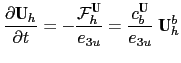
Both the surface momentum flux (wind stress) and the bottom momentum flux (bottom friction) enter the equations as a condition on the vertical diffusive flux. For the bottom boundary layer, one has:

$$A^{vm} \left( \partial {\textbf U}_h / \partial z \right) = {{\cal F}}_h^{\textbf U}$$ (10.27)

where ${\cal F}_h^{\textbf U}$ is represents the downward flux of horizontal momentum outside the logarithmic turbulent boundary layer (thickness of the order of 1 m in the ocean). How ${\cal F}_h^{\textbf U}$ influences the interior depends on the vertical resolution of the model near the bottom relative to the Ekman layer depth. For example, in order to obtain an Ekman layer depth $d = \sqrt{2\;A^{vm}} / f = 50$ m, one needs a vertical diffusion coefficient $A^{vm} = 0.125$ m$^2$s$^{-1}$ (for a Coriolis frequency $f = 10^{-4}$ m$^2$s$^{-1}$). With a background diffusion coefficient $A^{vm} = 10^{-4}$ m$^2$s$^{-1}$, the Ekman layer depth is only 1.4 m. When the vertical mixing coefficient is this small, using a flux condition is equivalent to entering the viscous forces (either wind stress or bottom friction) as a body force over the depth of the top or bottom model layer. To illustrate this, consider the equation for $u$ at $k$, the last ocean level:

$$\frac{\partial u_k}{\partial t} = \frac{1}{e_{3u}} \left[ \frac{A... ...lta_{k+1/2}\;[u] - {\cal F}^u_h \right] \approx - \frac{{\cal F}^u_{h}}{e_{3u}}$$ (10.28)

If the bottom layer thickness is 200 m, the Ekman transport will be distributed over that depth. On the other hand, if the vertical resolution is high (1 m or less) and a turbulent closure model is used, the turbulent Ekman layer will be represented explicitly by the model. However, the logarithmic layer is never represented in current primitive equation model applications: it is necessary to parameterize the flux ${\cal F}^u_h$. Two choices are available in NEMO: a linear and a quadratic bottom friction. Note that in both cases, the rotation between the interior velocity and the bottom friction is neglected in the present release of NEMO.

In the code, the bottom friction is imposed by adding the trend due to the bottom friction to the general momentum trend in dynbfr.F90. For the time-split surface pressure gradient algorithm, the momentum trend due to the barotropic component needs to be handled separately. For this purpose it is convenient to compute and store coefficients which can be simply combined with bottom velocities and geometric values to provide the momentum trend due to bottom friction. 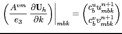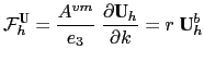These coefficients are computed in zdfbfr.F90 and generally take the form $c_b^{\textbf U}$ where:

$$\frac{\partial {\textbf U_h}}{\partial t} = - \frac{{\cal F}^{\textbf U}_{h}}{e_{3u}} = \frac{c_b^{\textbf U}}{e_{3u}} \;{\textbf U}_h^b$$ (10.29)

where $\textbf{U}_h^b = (u_b\;,\;v_b)$ is the near-bottom, horizontal, ocean velocity.

Linear Bottom Friction (nn_botfr = 0 or 1)

The linear bottom friction parameterisation (including the special case of a free-slip condition) assumes that the bottom friction is proportional to the interior velocity (i.e. the velocity of the last model level):

$${\cal F}_h^\textbf{U} = \frac{A^{vm}}{e_3} \; \frac{\partial \textbf{U}_h}{\partial k} = r \; \textbf{U}_h^b$$ (10.30)

where $r$ is a friction coefficient expressed in ms$^{-1}$. This coefficient is generally estimated by setting a typical decay time $\tau$ in the deep ocean, and setting $r = H / \tau$, where $H$ is the ocean depth. Commonly accepted values of $\tau$ are of the order of 100 to 200 days [Weatherly, 1984]. A value $\tau^{-1} = 10^{-7}$ s$^{-1}$ equivalent to 115 days, is usually used in quasi-geostrophic models. One may consider the linear friction as an approximation of quadratic friction, $r \approx 2\;C_D\;U_{av}$ (Gill [1982], Eq. 9.6.6). For example, with a drag coefficient $C_D = 0.002$, a typical speed of tidal currents of $U_{av} =0.1$ ms$^{-1}$, and assuming an ocean depth $H = 4000$ m, the resulting friction coefficient is $r = 4\;10^{-4}$ ms$^{-1}$. This is the default value used in NEMO. It corresponds to a decay time scale of 115 days. It can be changed by specifying rn_bfri1 (namelist parameter).

For the linear friction case the coefficients defined in the general expression (10.29) are:

$$\begin{split}c_b^u &= - r c_b^v &= - r \end{split}$$ (10.31)

When nn_botfr=1, the value of $r$ used is rn_bfri1. Setting nn_botfr=0 is equivalent to setting $r=0$ and leads to a free-slip bottom boundary condition. These values are assigned in zdfbfr.F90. From v3.2 onwards there is support for local enhancement of these values via an externally defined 2D mask array (ln_bfr2d=true) given in the bfr_coef.nc input NetCDF file. The mask values should vary from 0 to 1. Locations with a non-zero mask value will have the friction coefficient increased by $mask\_value$*rn_bfrien*rn_bfri1.

Non-Linear Bottom Friction (nn_botfr = 2)

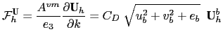
The non-linear bottom friction parameterisation assumes that the bottom friction is quadratic:

$${\cal F}_h^\textbf{U} = \frac{A^{vm}}{e_3 }\frac{\partial \textbf {U}_h }{\partial k}=C_D \;\sqrt {u_b ^2+v_b ^2+e_b } \;\; \textbf {U}_h^b$$ (10.32)

where $C_D$ is a drag coefficient, and $e_b$ a bottom turbulent kinetic energy due to tides, internal waves breaking and other short time scale currents. A typical value of the drag coefficient is $C_D = 10^{-3}$. As an example, the CME experiment [Tréguier, 1992] uses $C_D = 10^{-3}$ and $e_b = 2.5\;10^{-3}$m$^2$s$^{-2}$, while the FRAM experiment [Killworth, 1992] uses $C_D = 1.4\;10^{-3}$ and $e_b =2.5\;\;10^{-3}$m$^2$s$^{-2}$. The CME choices have been set as default values (rn_bfri2 and rn_bfeb2 namelist parameters).

As for the linear case, the bottom friction is imposed in the code by adding the trend due to the bottom friction to the general momentum trend in dynbfr.F90. For the non-linear friction case the terms computed in zdfbfr.F90 are:

$$\begin{split}c_b^u &= - \; C_D\;\left[ u^2 + \left(\bar{\bar{... ...ar{u}}^{i,j+1}\right)^2 + v^2 + e_b \right]^{1/2} \end{split}$$ (10.33)

The coefficients that control the strength of the non-linear bottom friction are initialised as namelist parameters: $C_D$= rn_bfri2, and $e_b$ =rn_bfeb2. Note for applications which treat tides explicitly a low or even zero value of rn_bfeb2 is recommended. From v3.2 onwards a local enhancement of $C_D$ is possible via an externally defined 2D mask array (ln_bfr2d=true). This works in the same way as for the linear bottom friction case with non-zero masked locations increased by $mask\_value$*rn_bfrien*rn_bfri2.

Log-layer Bottom Friction enhancement (nn_botfr = 2, ln_loglayer = .true.)

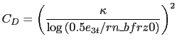
In the non-linear bottom friction case, the drag coefficient, $C_D$, can be optionally enhanced using a "law of the wall" scaling. If ln_loglayer = .true., $C_D$ is no longer constant but is related to the thickness of the last wet layer in each column by:

$$C_D = \left ( {\kappa \over {\rm log}\left ( 0.5e_{3t}/rn\_bfrz0 \right ) } \right )^2$$ (10.34)

where $\kappa$ is the von-Karman constant and rn_bfrz0 is a roughness length provided via the namelist.

For stability, the drag coefficient is bounded such that it is kept greater or equal to the base rn_bfri2 value and it is not allowed to exceed the value of an additional namelist parameter: rn_bfri2_max, i.e.:

$$rn\_bfri2 \leq C_D \leq rn\_bfri2\_max$$ (10.35)

Note also that a log-layer enhancement can also be applied to the top boundary friction if under ice-shelf cavities are in use (ln_isfcav=.true.). In this case, the relevant namelist parameters are rn_tfrz0, rn_tfri2 and rn_tfri2_max.

Bottom Friction stability considerations

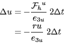
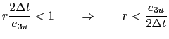
Some care needs to exercised over the choice of parameters to ensure that the implementation of bottom friction does not induce numerical instability. For the purposes of stability analysis, an approximation to (10.28) is:

$$\begin{split}\Delta u &= -\frac{{{\cal F}_h}^u}{e_{3u}}\;2 \rdt &= -\frac{ru}{e_{3u}}\;2\rdt \end{split}$$ (10.36)

where linear bottom friction and a leapfrog timestep have been assumed. To ensure that the bottom friction cannot reverse the direction of flow it is necessary to have:

$$\vert\Delta u\vert < \;\vert u\vert$$ (10.37)

which, using (10.36), gives:

$$r\frac{2\rdt}{e_{3u}} < 1 \qquad \Rightarrow \qquad r < \frac{e_{3u}}{2\rdt}$$ (10.38)

This same inequality can also be derived in the non-linear bottom friction case if a velocity of 1 m.s$^{-1}$ is assumed. Alternatively, this criterion can be rearranged to suggest a minimum bottom box thickness to ensure stability:

$$e_{3u} > 2\;r\;\rdt$$ (10.39)

which it may be necessary to impose if partial steps are being used. For example, if $\vert u\vert = 1$ m.s$^{-1}$, $rdt = 1800$ s, $r = 10^{-3}$ then $e_{3u}$ should be greater than 3.6 m. For most applications, with physically sensible parameters these restrictions should not be of concern. But caution may be necessary if attempts are made to locally enhance the bottom friction parameters. To ensure stability limits are imposed on the bottom friction coefficients both during initialisation and at each time step. Checks at initialisation are made in zdfbfr.F90 (assuming a 1 m.s$^{-1}$ velocity in the non-linear case). The number of breaches of the stability criterion are reported as well as the minimum and maximum values that have been set. The criterion is also checked at each time step, using the actual velocity, in dynbfr.F90. Values of the bottom friction coefficient are reduced as necessary to ensure stability; these changes are not reported.

Limits on the bottom friction coefficient are not imposed if the user has elected to handle the bottom friction implicitly (see §10.4.5). The number of potential breaches of the explicit stability criterion are still reported for information purposes.

Implicit Bottom Friction (ln_bfrimp$=$T)

An optional implicit form of bottom friction has been implemented to improve model stability. We recommend this option for shelf sea and coastal ocean applications, especially for split-explicit time splitting. This option can be invoked by setting ln_bfrimp to true in the nambfr namelist. This option requires ln_zdfexp to be false in the namzdf namelist.

This implementation is realised in dynzdf_imp.F90 and dynspg_ts.F90. In dynzdf_imp.F90, the bottom boundary condition is implemented implicitly.

$$\left.{\left( {\frac{A^{vm} }{e_3 } \frac{\partial \textbf{U}_h}... ...t)} \right\vert _{mbk} = \binom{c_{b}^{u}u^{n+1}_{mbk}}{c_{b}^{v}v^{n+1}_{mbk}}$$ (10.40)

where $mbk$ is the layer number of the bottom wet layer. superscript $n+1$ means the velocity used in the friction formula is to be calculated, so, it is implicit.

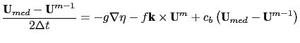
If split-explicit time splitting is used, care must be taken to avoid the double counting of the bottom friction in the 2-D barotropic momentum equations. As NEMO only updates the barotropic pressure gradient and Coriolis' forcing terms in the 2-D barotropic calculation, we need to remove the bottom friction induced by these two terms which has been included in the 3-D momentum trend and update it with the latest value. On the other hand, the bottom friction contributed by the other terms (e.g. the advection term, viscosity term) has been included in the 3-D momentum equations and should not be added in the 2-D barotropic mode.

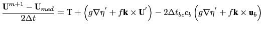
The implementation of the implicit bottom friction in dynspg_ts.F90 is done in two steps as the following:

$$\frac{\textbf{U}_{med}-\textbf{U}^{m-1}}{2\Delta t}=-g\nabla\eta-... ...tbf{k}\times\textbf{U}^{m}+c_{b} \left(\textbf{U}_{med}-\textbf{U}^{m-1}\right)$$ (10.41)

$$\frac{\textbf{U}^{m+1}-\textbf{U}_{med}}{2\Delta t}=\textbf{T}+ \... ...2\Delta t_{bc}c_{b}\left(g\nabla\eta^{'}+f\textbf{k}\times\textbf{u}_{b}\right)$$ (10.42)

where $\textbf{T}$ is the vertical integrated 3-D momentum trend. We assume the leap-frog time-stepping is used here. $\Delta t$ is the barotropic mode time step and $\Delta t_{bc}$ is the baroclinic mode time step. $c_{b}$ is the friction coefficient. $\eta$ is the sea surface level calculated in the barotropic loops while $\eta^{'}$ is the sea surface level used in the 3-D baroclinic mode. $\textbf{u}_{b}$ is the bottom layer horizontal velocity.

Bottom Friction with split-explicit time splitting (ln_bfrimp$=$F)

When calculating the momentum trend due to bottom friction in dynbfr.F90, the bottom velocity at the before time step is used. This velocity includes both the baroclinic and barotropic components which is appropriate when using either the explicit or filtered surface pressure gradient algorithms (key_ dynspg_exp or key_ dynspg_flt). Extra attention is required, however, when using split-explicit time stepping (key_ dynspg_ts). In this case the free surface equation is solved with a small time step rn_rdt/nn_baro, while the three dimensional prognostic variables are solved with the longer time step of rn_rdt seconds. The trend in the barotropic momentum due to bottom friction appropriate to this method is that given by the selected parameterisation ($i.e.$ linear or non-linear bottom friction) computed with the evolving velocities at each barotropic timestep.

In the case of non-linear bottom friction, we have elected to partially linearise the problem by keeping the coefficients fixed throughout the barotropic time-stepping to those computed in zdfbfr.F90 using the now timestep. This decision allows an efficient use of the $c_b^{\vect{U}}$ coefficients to:

1. On entry to dyn_spg_ts, remove the contribution of the before barotropic velocity to the bottom friction component of the vertically integrated momentum trend. Note the same stability check that is carried out on the bottom friction coefficient in dynbfr.F90 has to be applied here to ensure that the trend removed matches that which was added in dynbfr.F90.
2. At each barotropic step, compute the contribution of the current barotropic velocity to the trend due to bottom friction. Add this contribution to the vertically integrated momentum trend. This contribution is handled implicitly which eliminates the need to impose a stability criteria on the values of the bottom friction coefficient within the barotropic loop.

Note that the use of an implicit formulation within the barotropic loop for the bottom friction trend means that any limiting of the bottom friction coefficient in dynbfr.F90 does not adversely affect the solution when using split-explicit time splitting. This is because the major contribution to bottom friction is likely to come from the barotropic component which uses the unrestricted value of the coefficient. However, if the limiting is thought to be having a major effect (a more likely prospect in coastal and shelf seas applications) then the fully implicit form of the bottom friction should be used (see §10.4.5 ) which can be selected by setting ln_bfrimp $=$ true.

Otherwise, the implicit formulation takes the form:

$$\bar{U}^{t+ \rdt} = \; \left [ \bar{U}^{t-\rdt}\; + 2 \rdt\;RHS \right ] / \left [ 1 - 2 \rdt \;c_b^{u} / H_e \right ]$$ (10.43)

where $\bar U$ is the barotropic velocity, $H_e$ is the full depth (including sea surface height), $c_b^u$ is the bottom friction coefficient as calculated in zdf_bfr and $RHS$ represents all the components to the vertically integrated momentum trend except for that due to bottom friction.