Next: Internal wave-driven mixing (key_ Up: Vertical Ocean Physics (ZDF) Previous: Bottom and Top Friction Contents Index
!-----------------------------------------------------------------------
&namzdf_tmx    !   tidal mixing parameterization                        ("key_zdftmx")
!-----------------------------------------------------------------------
   rn_htmx     = 500.      !  vertical decay scale for turbulence (meters)
   rn_n2min    = 1.e-8     !  threshold of the Brunt-Vaisala frequency (s-1)
   rn_tfe      = 0.333     !  tidal dissipation efficiency
   rn_me       = 0.2       !  mixing efficiency
   ln_tmx_itf  = .true.    !  ITF specific parameterisation
   rn_tfe_itf  = 1.        !  ITF tidal dissipation efficiency
/
Options are defined through the namzdf_tmx namelist variables.
The parameterization of tidal mixing follows the general formulation for
the vertical eddy diffusivity proposed by St. Laurent et al. [2002] and
first introduced in an OGCM by [Simmons et al., 2004].
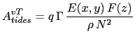
In this formulation an additional vertical diffusivity resulting from internal tide breaking,
![]() is expressed as a function of
is expressed as a function of ![]() , the energy transfer from barotropic
tides to baroclinic tides :
, the energy transfer from barotropic
tides to baroclinic tides :
The mixing efficiency of turbulence is set by ![]() (rn_me namelist parameter)
and is usually taken to be the canonical value of
(rn_me namelist parameter)
and is usually taken to be the canonical value of
![]() (Osborn 1980).
The tidal dissipation efficiency is given by the parameter
(Osborn 1980).
The tidal dissipation efficiency is given by the parameter ![]() (rn_tfe namelist parameter)
represents the part of the internal wave energy flux
(rn_tfe namelist parameter)
represents the part of the internal wave energy flux ![]() that is dissipated locally,
with the remaining
that is dissipated locally,
with the remaining ![]() radiating away as low mode internal waves and
contributing to the background internal wave field. A value of
radiating away as low mode internal waves and
contributing to the background internal wave field. A value of ![]() is typically used
St. Laurent et al. [2002].
The vertical structure function
is typically used
St. Laurent et al. [2002].
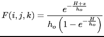
The vertical structure function ![]() models the distribution of the turbulent mixing in the vertical.
It is implemented as a simple exponential decaying upward away from the bottom,
with a vertical scale of
models the distribution of the turbulent mixing in the vertical.
It is implemented as a simple exponential decaying upward away from the bottom,
with a vertical scale of ![]() (rn_htmx namelist parameter, with a typical value of
(rn_htmx namelist parameter, with a typical value of ![]() ) [St. Laurent and Nash, 2004],
) [St. Laurent and Nash, 2004],
The associated vertical viscosity is calculated from the vertical
diffusivity assuming a Prandtl number of 1, ![]()
![]() .
In the limit of
.
In the limit of
![]() (or becoming negative), the vertical diffusivity
is capped at
(or becoming negative), the vertical diffusivity
is capped at
![]() and impose a lower limit on
and impose a lower limit on ![]() of rn_n2min
usually set to
of rn_n2min
usually set to
![]() . These bounds are usually rarely encountered.
. These bounds are usually rarely encountered.
The internal wave energy map, ![]() in (10.44), is derived
from a barotropic model of the tides utilizing a parameterization of the
conversion of barotropic tidal energy into internal waves.
The essential goal of the parameterization is to represent the momentum
exchange between the barotropic tides and the unrepresented internal waves
induced by the tidal flow over rough topography in a stratified ocean.
In the current version of NEMO, the map is built from the output of
the barotropic global ocean tide model MOG2D-G [Carrère and Lyard, 2003].
This model provides the dissipation associated with internal wave energy for the M2 and K1
tides component (Fig. 10.5). The S2 dissipation is simply approximated
as being
in (10.44), is derived
from a barotropic model of the tides utilizing a parameterization of the
conversion of barotropic tidal energy into internal waves.
The essential goal of the parameterization is to represent the momentum
exchange between the barotropic tides and the unrepresented internal waves
induced by the tidal flow over rough topography in a stratified ocean.
In the current version of NEMO, the map is built from the output of
the barotropic global ocean tide model MOG2D-G [Carrère and Lyard, 2003].
This model provides the dissipation associated with internal wave energy for the M2 and K1
tides component (Fig. 10.5). The S2 dissipation is simply approximated
as being ![]() of the M2 one. The internal wave energy is thus :
of the M2 one. The internal wave energy is thus :
![]() .
Its global mean value is
.
Its global mean value is ![]() TW, in agreement with independent estimates
[Egbert and Ray, 2001, Egbert and Ray, 2000].
TW, in agreement with independent estimates
[Egbert and Ray, 2001, Egbert and Ray, 2000].
When the Indonesian Through Flow (ITF) area is included in the model domain, a specific treatment of tidal induced mixing in this area can be used. It is activated through the namelist logical ln_tmx_itf, and the user must provide an input NetCDF file, mask_itf.nc , which contains a mask array defining the ITF area where the specific treatment is applied.
When ln_tmx_itf=true, the two key parameters ![]() and
and ![]() are adjusted following
the parameterisation developed by Koch-Larrouy et al. [2007]:
are adjusted following
the parameterisation developed by Koch-Larrouy et al. [2007]:
First, the Indonesian archipelago is a complex geographic region
with a series of large, deep, semi-enclosed basins connected via
numerous narrow straits. Once generated, internal tides remain
confined within this semi-enclosed area and hardly radiate away.
Therefore all the internal tides energy is consumed within this area.
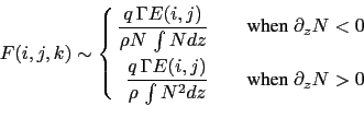
So it is assumed that ![]() ,
, ![]() all the energy generated is available for mixing.
Note that for test purposed, the ITF tidal dissipation efficiency is a
namelist parameter (rn_tfe_itf). A value of
all the energy generated is available for mixing.
Note that for test purposed, the ITF tidal dissipation efficiency is a
namelist parameter (rn_tfe_itf). A value of ![]() or close to is
this recommended for this parameter.
or close to is
this recommended for this parameter.
Second, the vertical structure function, ![]() , is no more associated
with a bottom intensification of the mixing, but with a maximum of
energy available within the thermocline. Koch-Larrouy et al. [2007]
have suggested that the vertical distribution of the energy dissipation
proportional to
, is no more associated
with a bottom intensification of the mixing, but with a maximum of
energy available within the thermocline. Koch-Larrouy et al. [2007]
have suggested that the vertical distribution of the energy dissipation
proportional to ![]() below the core of the thermocline and to
below the core of the thermocline and to ![]() above.
The resulting
above.
The resulting ![]() is:
is:
Averaged over the ITF area, the resulting tidal mixing coefficient is
![]() ,
which agrees with the independent estimates inferred from observations.
Introduced in a regional OGCM, the parameterization improves the water mass
characteristics in the different Indonesian seas, suggesting that the horizontal
and vertical distributions of the mixing are adequately prescribed
[Koch-Larrouy et al., 2008a, Koch-Larrouy et al., 2007, Koch-Larrouy et al., 2008b].
Note also that such a parameterisation has a significant impact on the behaviour
of global coupled GCMs [Koch-Larrouy et al., 2010].
,
which agrees with the independent estimates inferred from observations.
Introduced in a regional OGCM, the parameterization improves the water mass
characteristics in the different Indonesian seas, suggesting that the horizontal
and vertical distributions of the mixing are adequately prescribed
[Koch-Larrouy et al., 2008a, Koch-Larrouy et al., 2007, Koch-Larrouy et al., 2008b].
Note also that such a parameterisation has a significant impact on the behaviour
of global coupled GCMs [Koch-Larrouy et al., 2010].
Gurvan Madec and the NEMO Team
NEMO European Consortium2017-02-17
![\includegraphics[width=0.90\textwidth]{Fig_ZDF_M2_K1_tmx}](img1140.png)