Vertical diffusion term (dynzdf.F90)

!-----------------------------------------------------------------------
&namzdf        !   vertical physics
!-----------------------------------------------------------------------
   rn_avm0     =   1.2e-4  !  vertical eddy viscosity   [m2/s]          (background Kz if not "key_zdfcst")
   rn_avt0     =   1.2e-5  !  vertical eddy diffusivity [m2/s]          (background Kz if not "key_zdfcst")
   nn_avb      =    0      !  profile for background avt & avm (=1) or not (=0)
   nn_havtb    =    0      !  horizontal shape for avtb (=1) or not (=0)
   ln_zdfevd   = .true.    !  enhanced vertical diffusion (evd) (T) or not (F)
   nn_evdm     =    0      !  evd apply on tracer (=0) or on tracer and momentum (=1)
   rn_avevd    =  100.     !  evd mixing coefficient [m2/s]
   ln_zdfnpc   = .false.   !  Non-Penetrative Convective algorithm (T) or not (F)
   nn_npc      =    1            !  frequency of application of npc
   nn_npcp     =  365            !  npc control print frequency
   ln_zdfexp   = .false.   !  time-stepping: split-explicit (T) or implicit (F) time stepping
   nn_zdfexp   =    3            !  number of sub-timestep for ln_zdfexp=T
/

Options are defined through the namzdf namelist variables. The large vertical diffusion coefficient found in the surface mixed layer together with high vertical resolution implies that in the case of explicit time stepping there would be too restrictive a constraint on the time step. Two time stepping schemes can be used for the vertical diffusion term : $(a)$ a forward time differencing scheme (ln_zdfexp=true) using a time splitting technique (nn_zdfexp $>$ 1) or $(b)$ a backward (or implicit) time differencing scheme (ln_zdfexp=false) (see §3). Note that namelist variables ln_zdfexp and nn_zdfexp apply to both tracers and dynamics.

The formulation of the vertical subgrid scale physics is the same whatever the vertical coordinate is. The vertical diffusion operators given by (2.34) take the following semi-discrete space form:

$$\left\{ \begin{aligned}D_u^{vm} &\equiv \frac{1}{e_{3u}} \del... ...e_{3vw} } \delta _{k+1/2} [ v ] \right] \end{aligned} \right.$$

where $A_{uw}^{vm}$ and $A_{vw}^{vm}$ are the vertical eddy viscosity and diffusivity coefficients. The way these coefficients are evaluated depends on the vertical physics used (see §10).

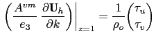
The surface boundary condition on momentum is the stress exerted by the wind. At the surface, the momentum fluxes are prescribed as the boundary condition on the vertical turbulent momentum fluxes,

$$\left.{\left( {\frac{A^{vm} }{e_3 } \frac{\partial \textbf{U}_h}... ...l k}} \right)} \right\vert _{z=1} = \frac{1}{\rho _o} \binom{\tau _u}{\tau _v }$$ (6.28)

where $\left( \tau _u ,\tau _v \right)$ are the two components of the wind stress vector in the (i,j) coordinate system. The high mixing coefficients in the surface mixed layer ensure that the surface wind stress is distributed in the vertical over the mixed layer depth. If the vertical mixing coefficient is small (when no mixed layer scheme is used) the surface stress enters only the top model level, as a body force. The surface wind stress is calculated in the surface module routines (SBC, see Chap.7)

The turbulent flux of momentum at the bottom of the ocean is specified through a bottom friction parameterisation (see §10.4)