Next: Coriolis and Advection: flux Up: Ocean Dynamics (DYN) Previous: Sea surface height and Contents Index
!-----------------------------------------------------------------------
&namdyn_adv    !   formulation of the momentum advection
!-----------------------------------------------------------------------
   ln_dynadv_vec = .true.  !  vector form (T) or flux form (F)
   nn_dynkeg     = 0       ! scheme for grad(KE): =0   C2  ;  =1   Hollingsworth correction
   ln_dynadv_cen2= .false. !  flux form - 2nd order centered scheme
   ln_dynadv_ubs = .false. !  flux form - 3rd order UBS      scheme
   ln_dynzad_zts = .false. !  Use (T) sub timestepping for vertical momentum advection
/
The vector invariant form of the momentum equations (ln_dynhpg_vec = true) is the one most
often used in applications of the NEMO ocean model. The flux form option (ln_dynhpg_vec =false)
(see next section) has been present since version ![]() .
Options are defined through the namdyn_adv namelist variables.
Coriolis and momentum advection terms are evaluated using a leapfrog scheme,
.
Options are defined through the namdyn_adv namelist variables.
Coriolis and momentum advection terms are evaluated using a leapfrog scheme,
![]() the velocity appearing in these expressions is centred in time (now velocity).
At the lateral boundaries either free slip, no slip or partial slip boundary
conditions are applied following Chap.8.
the velocity appearing in these expressions is centred in time (now velocity).
At the lateral boundaries either free slip, no slip or partial slip boundary
conditions are applied following Chap.8.
!-----------------------------------------------------------------------
&namdyn_vor    !   option of physics/algorithm (not control by CPP keys)
!-----------------------------------------------------------------------
   ln_dynvor_ene = .false. !  enstrophy conserving scheme
   ln_dynvor_ens = .false. !  energy conserving scheme
   ln_dynvor_mix = .false. !  mixed scheme
   ln_dynvor_een = .true.  !  energy & enstrophy scheme
   ln_dynvor_een_old = .false.  !  energy & enstrophy scheme - original formulation
/
Options are defined through the namdyn_vor namelist variables. Four discretisations of the vorticity term (ln_dynvor_xxx=true) are available: conserving potential enstrophy of horizontally non-divergent flow (ENS scheme) ; conserving horizontal kinetic energy (ENE scheme) ; conserving potential enstrophy for the relative vorticity term and horizontal kinetic energy for the planetary vorticity term (MIX scheme) ; or conserving both the potential enstrophy of horizontally non-divergent flow and horizontal kinetic energy (EEN scheme) (see Appendix C.5). In the case of ENS, ENE or MIX schemes the land sea mask may be slightly modified to ensure the consistency of vorticity term with analytical equations (ln_dynvor_con=true). The vorticity terms are all computed in dedicated routines that can be found in the dynvor.F90 module.
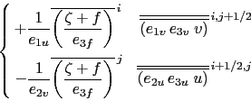
In the enstrophy conserving case (ENS scheme), the discrete formulation of the
vorticity term provides a global conservation of the enstrophy
(
![]() in
in ![]() -coordinates) for a horizontally non-divergent
flow (
-coordinates) for a horizontally non-divergent
flow (![]()
![]() =0), but does not conserve the total kinetic energy. It is given by:
=0), but does not conserve the total kinetic energy. It is given by:
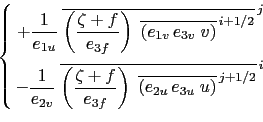
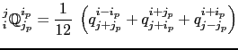
The kinetic energy conserving scheme (ENE scheme) conserves the global kinetic energy but not the global enstrophy. It is given by:
For the mixed energy/enstrophy conserving scheme (MIX scheme), a mixture of the two previous schemes is used. It consists of the ENS scheme (C.13) for the relative vorticity term, and of the ENE scheme (6.6) applied to the planetary vorticity term.
In both the ENS and ENE schemes, it is apparent that the combination of ![]() and
and ![]() averages of the velocity allows for the presence of grid point oscillation structures
that will be invisible to the operator. These structures are computational modes
that will be at least partly damped by the momentum diffusion operator (
averages of the velocity allows for the presence of grid point oscillation structures
that will be invisible to the operator. These structures are computational modes
that will be at least partly damped by the momentum diffusion operator (![]() the
subgrid-scale advection), but not by the resolved advection term. The ENS and ENE schemes
therefore do not contribute to dump any grid point noise in the horizontal velocity field.
Such noise would result in more noise in the vertical velocity field, an undesirable feature.
This is a well-known characteristic of
the
subgrid-scale advection), but not by the resolved advection term. The ENS and ENE schemes
therefore do not contribute to dump any grid point noise in the horizontal velocity field.
Such noise would result in more noise in the vertical velocity field, an undesirable feature.
This is a well-known characteristic of ![]() -grid discretization where
-grid discretization where ![]() and
and 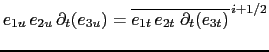 are located
at different grid points, a price worth paying to avoid a double averaging in the pressure
gradient term as in the
are located
at different grid points, a price worth paying to avoid a double averaging in the pressure
gradient term as in the ![]() -grid.
-grid.
A very nice solution to the problem of double averaging was proposed by Arakawa and Hsu [1990]. The idea is to get rid of the double averaging by considering triad combinations of vorticity. It is noteworthy that this solution is conceptually quite similar to the one proposed by [Griffies et al., 1998] for the discretization of the iso-neutral diffusion operator (see App.C).
The Arakawa and Hsu [1990] vorticity advection scheme for a single layer is modified
for spherical coordinates as described by Arakawa and Lamb [1981] to obtain the EEN scheme.
First consider the discrete expression of the potential vorticity, ![]() , defined at an
, defined at an ![]() -point:
-point:
![\includegraphics[width=0.70\textwidth]{Fig_DYN_een_triad}](img660.png)
|
A key point in (6.9) is how the averaging in the i- and j- directions is made.
It uses the sum of masked t-point vertical scale factor divided either
by the sum of the four t-point masks (ln_dynvor_een_old = false),
or just by ![]() (ln_dynvor_een_old = true).
The latter case preserves the continuity of
(ln_dynvor_een_old = true).
The latter case preserves the continuity of ![]() when one or more of the neighbouring
when one or more of the neighbouring ![]() tends to zero and extends by continuity the value of
tends to zero and extends by continuity the value of ![]() into the land areas.
This case introduces a sub-grid-scale topography at f-points (with a systematic reduction of
into the land areas.
This case introduces a sub-grid-scale topography at f-points (with a systematic reduction of ![]() when a model level intercept the bathymetry) that tends to reinforce the topostrophy of the flow
(
when a model level intercept the bathymetry) that tends to reinforce the topostrophy of the flow
(![]() the tendency of the flow to follow the isobaths) [Penduff et al., 2007].
the tendency of the flow to follow the isobaths) [Penduff et al., 2007].
Next, the vorticity triads,
![]() can be defined at a
can be defined at a ![]() -point as
the following triad combinations of the neighbouring potential vorticities defined at f-points
(Fig. 6.1):
-point as
the following triad combinations of the neighbouring potential vorticities defined at f-points
(Fig. 6.1):
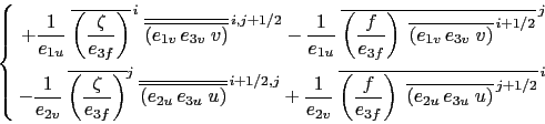
Finally, the vorticity terms are represented as:
This EEN scheme in fact combines the conservation properties of the ENS and ENE schemes.
It conserves both total energy and potential enstrophy in the limit of horizontally
nondivergent flow (![]()
![]() =0) (see Appendix C.5).
Applied to a realistic ocean configuration, it has been shown that it leads to a significant
reduction of the noise in the vertical velocity field [Le Sommer et al., 2009].
Furthermore, used in combination with a partial steps representation of bottom topography,
it improves the interaction between current and topography, leading to a larger
topostrophy of the flow [Penduff et al., 2007, Barnier et al., 2006].
=0) (see Appendix C.5).
Applied to a realistic ocean configuration, it has been shown that it leads to a significant
reduction of the noise in the vertical velocity field [Le Sommer et al., 2009].
Furthermore, used in combination with a partial steps representation of bottom topography,
it improves the interaction between current and topography, leading to a larger
topostrophy of the flow [Penduff et al., 2007, Barnier et al., 2006].
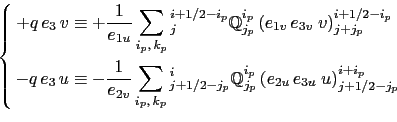
As demonstrated in Appendix C, there is a single discrete formulation of the kinetic energy gradient term that, together with the formulation chosen for the vertical advection (see below), conserves the total kinetic energy:
The discrete formulation of the vertical advection, together with the formulation chosen for the gradient of kinetic energy (KE) term, conserves the total kinetic energy. Indeed, the change of KE due to the vertical advection is exactly balanced by the change of KE due to the gradient of KE (see Appendix C).
Gurvan Madec and the NEMO Team
NEMO European Consortium2017-02-17

![\begin{equation*}\left\{ \begin{aligned}-\frac{1}{2 \; e_{1u} } & \delta _{i+1...
...{u^2}^{ i} + \overline{v^2}^{ j}} \right] \end{aligned} \right.\end{equation*}](img672.png)
![\begin{equation*}\left\{ \begin{aligned}-\frac{1} {e_{1u} e_{2u} e_{3u}} & \o...
...\;\delta _{k+1/2} \left[ u \right] }^{ k} \end{aligned} \right.\end{equation*}](img673.png)