Tracer Advection (traadv.F90)

!-----------------------------------------------------------------------
&namtra_adv    !   advection scheme for tracer
!-----------------------------------------------------------------------
   ln_traadv_cen2   =  .false.   !  2nd order centered scheme
   ln_traadv_tvd    =  .true.    !  TVD scheme
   ln_traadv_muscl  =  .false.   !  MUSCL scheme
   ln_traadv_muscl2 =  .false.   !  MUSCL2 scheme + cen2 at boundaries
   ln_traadv_ubs    =  .false.   !  UBS scheme
   ln_traadv_qck    =  .false.   !  QUICKEST scheme
   ln_traadv_msc_ups=  .false.   !  use upstream scheme within muscl
   ln_traadv_tvd_zts=  .false.  !  TVD scheme with sub-timestepping of vertical tracer advection
/

The advection tendency of a tracer in flux form is the divergence of the advective fluxes. Its discrete expression is given by :

$$ADV_\tau =-\frac{1}{b_t} \left( \;\delta _i \left[ e_{2u} e_{3u}... ... _v \right] \; \right) -\frac{1}{e_{3t}} \;\delta _k \left[ w\; \tau _w \right]$$ (5.1)

where $\tau$ is either T or S, and $b_t= e_{1t} e_{2t} e_{3t}$ is the volume of $T$-cells. The flux form in (5.1) implicitly requires the use of the continuity equation. Indeed, it is obtained by using the following equality : $\nabla \cdot \left( \vect{U} T \right)=\vect{U} \cdot \nabla T$ which results from the use of the continuity equation, $\nabla \cdot \vect{U}=0$ or $\partial _t e_3 + e_3\;\nabla \cdot \vect{U}=0$ in constant volume or variable volume case, respectively. Therefore it is of paramount importance to design the discrete analogue of the advection tendency so that it is consistent with the continuity equation in order to enforce the conservation properties of the continuous equations. In other words, by replacing $\tau$ by the number 1 in (5.1) we recover the discrete form of the continuity equation which is used to calculate the vertical velocity.

Figure 5.1: Schematic representation of some ways used to evaluate the tracer value at $u$-point and the amount of tracer exchanged between two neighbouring grid points. Upsteam biased scheme (ups): the upstream value is used and the black area is exchanged. Piecewise parabolic method (ppm): a parabolic interpolation is used and the black and dark grey areas are exchanged. Monotonic upstream scheme for conservative laws (muscl): a parabolic interpolation is used and black, dark grey and grey areas are exchanged. Second order scheme (cen2): the mean value is used and black, dark grey, grey and light grey areas are exchanged. Note that this illustration does not include the flux limiter used in ppm and muscl schemes.

The key difference between the advection schemes available in NEMO is the choice made in space and time interpolation to define the value of the tracer at the velocity points (Fig. 5.1).

Along solid lateral and bottom boundaries a zero tracer flux is automatically specified, since the normal velocity is zero there. At the sea surface the boundary condition depends on the type of sea surface chosen:

linear free surface:

the first level thickness is constant in time: the vertical boundary condition is applied at the fixed surface $z=0$ rather than on the moving surface $z=\eta$. There is a non-zero advective flux which is set for all advection schemes as $\left. {\tau _w } \right\vert _{k=1/2} =T_{k=1}$, $i.e.$ the product of surface velocity (at $z=0$) by the first level tracer value.

non-linear free surface:

(key_ vvl is defined) convergence/divergence in the first ocean level moves the free surface up/down. There is no tracer advection through it so that the advective fluxes through the surface are also zero

In all cases, this boundary condition retains local conservation of tracer. Global conservation is obtained in non-linear free surface case, but not in the linear free surface case. Nevertheless, in the latter case, it is achieved to a good approximation since the non-conservative term is the product of the time derivative of the tracer and the free surface height, two quantities that are not correlated (see §2.2.2, and also Roullet and Madec [2000], Griffies et al. [2001], Campin et al. [2004]).

The velocity field that appears in (5.1) and () is the centred (now) effective ocean velocity, $i.e.$ the eulerian velocity (see Chap. 6) plus the eddy induced velocity (eiv) and/or the mixed layer eddy induced velocity (eiv) when those parameterisations are used (see Chap. 9).

The choice of an advection scheme is made in the nam_traadv namelist, by setting to true one and only one of the logicals ln_traadv_xxx. The corresponding code can be found in the traadv_xxx.F90 module, where xxx is a 3 or 4 letter acronym corresponding to each scheme. Details of the advection schemes are given below. The choice of an advection scheme is a complex matter which depends on the model physics, model resolution, type of tracer, as well as the issue of numerical cost.

Note that (1) cen2 and TVD schemes require an explicit diffusion operator while the other schemes are diffusive enough so that they do not require additional diffusion ; (2) cen2, MUSCL2, and UBS are not positive schemes ^5.1, implying that false extrema are permitted. Their use is not recommended on passive tracers ; (3) It is recommended that the same advection-diffusion scheme is used on both active and passive tracers. Indeed, if a source or sink of a passive tracer depends on an active one, the difference of treatment of active and passive tracers can create very nice-looking frontal structures that are pure numerical artefacts. Nevertheless, most of our users set a different treatment on passive and active tracers, that's the reason why this possibility is offered. We strongly suggest them to perform a sensitivity experiment using a same treatment to assess the robustness of their results.

$2^{nd}$ order centred scheme (cen2) (ln_traadv_cen2=true)

In the centred second order formulation, the tracer at velocity points is evaluated as the mean of the two neighbouring $T$-point values. For example, in the $i$-direction :

$$\tau _u^{cen2} =\overline T ^{i+1/2}$$ (5.2)

The scheme is non diffusive ($i.e.$ it conserves the tracer variance, $\tau^2)$ but dispersive ($i.e.$ it may create false extrema). It is therefore notoriously noisy and must be used in conjunction with an explicit diffusion operator to produce a sensible solution. The associated time-stepping is performed using a leapfrog scheme in conjunction with an Asselin time-filter, so $T$ in (5.2) is the now tracer value. The centered second order advection is computed in the traadv_cen2.F90 module. In this module, it is advantageous to combine the cen2 scheme with an upstream scheme in specific areas which require a strong diffusion in order to avoid the generation of false extrema. These areas are the vicinity of large river mouths, some straits with coarse resolution, and the vicinity of ice cover area ($i.e.$ when the ocean temperature is close to the freezing point). This combined scheme has been included for specific grid points in the ORCA2 configuration only. This is an obsolescent feature as the recommended advection scheme for the ORCA configuration is TVD (see §5.1.2).

Note that using the cen2 scheme, the overall tracer advection is of second order accuracy since both (5.1) and (5.2) have this order of accuracy.

Total Variance Dissipation scheme (TVD) (ln_traadv_tvd=true)

In the Total Variance Dissipation (TVD) formulation, the tracer at velocity points is evaluated using a combination of an upstream and a centred scheme. For example, in the $i$-direction :

$$\begin{split}\tau _u^{ups}&= \begin{cases}T_{i+1} & \text{if ... ...u \;\left( {\tau _u^{cen2} -\tau _u^{ups} } \right) \end{split}$$ (5.3)

where $c_u$ is a flux limiter function taking values between 0 and 1. There exist many ways to define $c_u$, each corresponding to a different total variance decreasing scheme. The one chosen in NEMO is described in Zalesak [1979]. $c_u$ only departs from $1$ when the advective term produces a local extremum in the tracer field. The resulting scheme is quite expensive but positive. It can be used on both active and passive tracers. This scheme is tested and compared with MUSCL and the MPDATA scheme in Lévy et al. [2001]; note that in this paper it is referred to as "FCT" (Flux corrected transport) rather than TVD. The TVD scheme is implemented in the traadv_tvd.F90 module.

For stability reasons (see §3), $\tau _u^{cen2}$ is evaluated in (5.3) using the now tracer while $\tau _u^{ups}$ is evaluated using the before tracer. In other words, the advective part of the scheme is time stepped with a leap-frog scheme while a forward scheme is used for the diffusive part.

An additional option has been added controlled by ln_traadv_tvd_zts. By setting this logical to true, a TVD scheme is used on both horizontal and vertical direction, but on the latter, a split-explicit time stepping is used, with 5 sub-timesteps. This option can be useful when the value of the timestep is limited by vertical advection [Lemarié et al., 2015]. Note that in this case, a similar split-explicit time stepping should be used on vertical advection of momentum to ensure a better stability (see ln_dynzad_zts in §6.2.3).

Monotone Upstream Scheme for Conservative Laws (MUSCL) (ln_traadv_muscl=T)

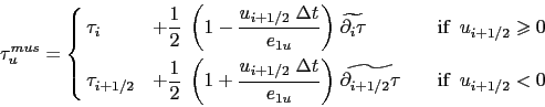
The Monotone Upstream Scheme for Conservative Laws (MUSCL) has been implemented by Lévy et al. [2001]. In its formulation, the tracer at velocity points is evaluated assuming a linear tracer variation between two $T$-points (Fig.5.1). For example, in the $i$-direction :

$$\tau _u^{mus} = \left\{ \begin{aligned}&\tau _i &+ \frac{1}{2} ... ...l_{i+1/2} \tau } & \text{if }\;u_{i+1/2} <0 \end{aligned} \right.$$

where $\widetilde{\partial _i \tau}$ is the slope of the tracer on which a limitation is imposed to ensure the positive character of the scheme.

The time stepping is performed using a forward scheme, that is the before tracer field is used to evaluate $\tau _u^{mus}$.

For an ocean grid point adjacent to land and where the ocean velocity is directed toward land, two choices are available: an upstream flux (ln_traadv_muscl=true) or a second order flux (ln_traadv_muscl2=true). Note that the latter choice does not ensure the positive character of the scheme. Only the former can be used on both active and passive tracers. The two MUSCL schemes are implemented in the traadv_tvd.F90 and traadv_tvd2.F90 modules.

Note that when using npln_traadv_msc_ups = true in addition to ln_traadv_muscl=true, the MUSCL fluxes are replaced by upstream fluxes in vicinity of river mouths.

Upstream-Biased Scheme (UBS) (ln_traadv_ubs=true)

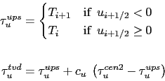
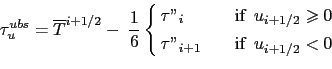
The UBS advection scheme is an upstream-biased third order scheme based on an upstream-biased parabolic interpolation. It is also known as the Cell Averaged QUICK scheme (Quadratic Upstream Interpolation for Convective Kinematics). For example, in the $i$-direction :

$$\tau _u^{ubs} =\overline T ^{i+1/2}-\;\frac{1}{6} \left\{ \begi... ...u''_{i+1} & \quad \text{if } u_{i+1/2} < 0 \end{aligned} \right.$$

where $\tau ''_i =\delta _i \left[ {\delta _{i+1/2} \left[ \tau \right]} \right]$.

This results in a dissipatively dominant (i.e. hyper-diffusive) truncation error [Shchepetkin and McWilliams, 2005]. The overall performance of the advection scheme is similar to that reported in Farrow and Stevens [1995]. It is a relatively good compromise between accuracy and smoothness. It is not a positive scheme, meaning that false extrema are permitted, but the amplitude of such are significantly reduced over the centred second order method. Nevertheless it is not recommended that it should be applied to a passive tracer that requires positivity.

The intrinsic diffusion of UBS makes its use risky in the vertical direction where the control of artificial diapycnal fluxes is of paramount importance. Therefore the vertical flux is evaluated using the TVD scheme when ln_traadv_ubs=true.

For stability reasons (see §3), the first term in (5.5) (which corresponds to a second order centred scheme) is evaluated using the now tracer (centred in time) while the second term (which is the diffusive part of the scheme), is evaluated using the before tracer (forward in time). This choice is discussed by Webb et al. [1998] in the context of the QUICK advection scheme. UBS and QUICK schemes only differ by one coefficient. Replacing 1/6 with 1/8 in (5.5) leads to the QUICK advection scheme [Webb et al., 1998]. This option is not available through a namelist parameter, since the 1/6 coefficient is hard coded. Nevertheless it is quite easy to make the substitution in the traadv_ubs.F90 module and obtain a QUICK scheme.

Four different options are possible for the vertical component used in the UBS scheme. $\tau _w^{ubs}$ can be evaluated using either (a) a centred $2^{nd}$ order scheme, or (b) a TVD scheme, or (c) an interpolation based on conservative parabolic splines following the Shchepetkin and McWilliams [2005] implementation of UBS in ROMS, or (d) a UBS. The $3^{rd}$ case has dispersion properties similar to an eighth-order accurate conventional scheme. The current reference version uses method b)

Note that :

(1) When a high vertical resolution $O(1m)$ is used, the model stability can be controlled by vertical advection (not vertical diffusion which is usually solved using an implicit scheme). Computer time can be saved by using a time-splitting technique on vertical advection. Such a technique has been implemented and validated in ORCA05 with 301 levels. It is not available in the current reference version.

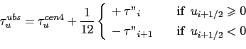
(2) It is straightforward to rewrite (5.5) as follows:

$$\tau _u^{ubs} = \tau _u^{cen4} + \frac{1}{12} \left\{ \begin{al... ...u''_{i+1} & \quad \text{if } u_{i+1/2} < 0 \end{aligned} \right.$$

or equivalently

$$u_{i+1/2} \tau _u^{ubs} =u_{i+1/2} \overline{ T - \frac{1}{6}... ...2} - \frac{1}{2} \vert u\vert _{i+1/2} \;\frac{1}{6} \;\delta_{i+1/2}[\tau''_i]$$ (5.7)

(5.6) has several advantages. Firstly, it clearly reveals that the UBS scheme is based on the fourth order scheme to which an upstream-biased diffusion term is added. Secondly, this emphasises that the $4^{th}$ order part (as well as the $2^{nd}$ order part as stated above) has to be evaluated at the now time step using (5.5). Thirdly, the diffusion term is in fact a biharmonic operator with an eddy coefficient which is simply proportional to the velocity: $A_u^{lm}= - \frac{1}{12} {e_{1u}}^3 \vert u\vert$. Note that NEMO v3.4 still uses (5.5), not (5.6).

QUICKEST scheme (QCK) (ln_traadv_qck=true)

The Quadratic Upstream Interpolation for Convective Kinematics with Estimated Streaming Terms (QUICKEST) scheme proposed by Leonard [1979] is the third order Godunov scheme. It is associated with the ULTIMATE QUICKEST limiter [Leonard, 1991]. It has been implemented in NEMO by G. Reffray (MERCATOR-ocean) and can be found in the traadv_qck.F90 module. The resulting scheme is quite expensive but positive. It can be used on both active and passive tracers. However, the intrinsic diffusion of QCK makes its use risky in the vertical direction where the control of artificial diapycnal fluxes is of paramount importance. Therefore the vertical flux is evaluated using the CEN2 scheme. This no longer guarantees the positivity of the scheme. The use of TVD in the vertical direction (as for the UBS case) should be implemented to restore this property.

Footnotes

... schemes^5.1

negative values can appear in an initially strictly positive tracer field which is advected