Sea surface height and diagnostic variables ($\eta$, $\zeta$, $\chi$, $w$)

Horizontal divergence and relative vorticity (divcur.F90)

The vorticity is defined at an $f$-point ($i.e.$ corner point) as follows:

$$\zeta =\frac{1}{e_{1f} e_{2f} }\left( {\;\delta _{i+1/2} \left[ {e_{2v}\;v} \right] -\delta _{j+1/2} \left[ {e_{1u}\;u} \right]\;} \right)$$ (6.1)

The horizontal divergence is defined at a $T$-point. It is given by:

$$\chi =\frac{1}{e_{1t} e_{2t} e_{3t} } \left( {\delta _i \left[ {e_{2u} e_{3u} u} \right] +\delta _j \left[ {e_{1v} e_{3v} v} \right]} \right)$$ (6.2)

Note that although the vorticity has the same discrete expression in $z$- and $s$-coordinates, its physical meaning is not identical. $\zeta$ is a pseudo vorticity along $s$-surfaces (only pseudo because $(u,v)$ are still defined along geopotential surfaces, but are not necessarily defined at the same depth).

The vorticity and divergence at the before step are used in the computation of the horizontal diffusion of momentum. Note that because they have been calculated prior to the Asselin filtering of the before velocities, the before vorticity and divergence arrays must be included in the restart file to ensure perfect restartability. The vorticity and divergence at the now time step are used for the computation of the nonlinear advection and of the vertical velocity respectively.

Horizontal divergence and relative vorticity (sshwzv.F90)

The sea surface height is given by :

$$\begin{aligned}\frac{\partial \eta }{\partial t} &\equiv \frac{... ...s_k {\chi e_{3t}} - \frac{\textit{emp}}{\rho _w } \end{aligned}$$

where emp is the surface freshwater budget (evaporation minus precipitation), expressed in Kg/m$^2$/s (which is equal to mm/s), and $\rho _w$=1,035 Kg/m$^3$ is the reference density of sea water (Boussinesq approximation). If river runoff is expressed as a surface freshwater flux (see §7) then emp can be written as the evaporation minus precipitation, minus the river runoff. The sea-surface height is evaluated using exactly the same time stepping scheme as the tracer equation (5.24): a leapfrog scheme in combination with an Asselin time filter, $i.e.$ the velocity appearing in (6.3) is centred in time (now velocity). This is of paramount importance. Replacing $T$ by the number $1$ in the tracer equation and summing over the water column must lead to the sea surface height equation otherwise tracer content will not be conserved [Griffies et al., 2001, Leclair and Madec, 2009].

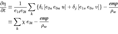
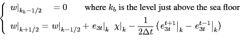
The vertical velocity is computed by an upward integration of the horizontal divergence starting at the bottom, taking into account the change of the thickness of the levels :

$$\left\{ \begin{aligned}&\left. w \right\vert _{k_b-1/2} \quad= ... ... \left. e_{3t}^{t-1}\right\vert _{k}\right) \end{aligned} \right.$$

In the case of a non-linear free surface (key_ vvl), the top vertical velocity is $-\textit{emp}/\rho_w$, as changes in the divergence of the barotropic transport are absorbed into the change of the level thicknesses, re-orientated downward. In the case of a linear free surface, the time derivative in (6.4) disappears. The upper boundary condition applies at a fixed level $z=0$. The top vertical velocity is thus equal to the divergence of the barotropic transport ($i.e.$ the first term in the right-hand-side of (6.3)).

Note also that whereas the vertical velocity has the same discrete expression in $z$- and $s$-coordinates, its physical meaning is not the same: in the second case, $w$ is the velocity normal to the $s$-surfaces. Note also that the $k$-axis is re-orientated downwards in the FORTRAN code compared to the indexing used in the semi-discrete equations such as (6.4) (see §4.1.3).