Next: Discrete total energy conservation Up: Discrete Invariants of the Previous: Continuous conservation Contents Index
The discrete form of the total energy conservation, (C.3), is given by:
 |
Substituting the discrete expression of the time derivative of the velocity either in vector invariant, leads to the discrete equivalent of the four equations (C.6).
Let ![]() , located at
, located at ![]() -points, be either the relative (
-points, be either the relative (
![]() ), or
the planetary (
), or
the planetary (
![]() ), or the total potential vorticity (
), or the total potential vorticity (
 ).
Two discretisation of the vorticity term (ENE and EEN) allows the conservation of
the kinetic energy.
).
Two discretisation of the vorticity term (ENE and EEN) allows the conservation of
the kinetic energy.
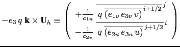
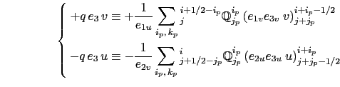
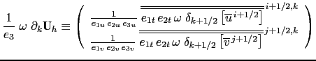
For the ENE scheme, the two components of the vorticity term are given by :
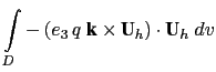 |
This formulation does not conserve the enstrophy but it does conserve the total kinetic energy. Indeed, the kinetic energy tendency associated to the vorticity term and averaged over the ocean domain can be transformed as follows:
 |
||||
 |
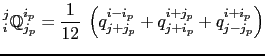
With the EEN scheme, the vorticity terms are represented as:
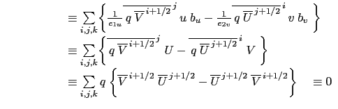
This formulation does conserve the total kinetic energy. Indeed,
 |
||||
|
||||
|
Expending the summation on
| ||||
 |
 |
|||
 |
||||
 |
||||
|
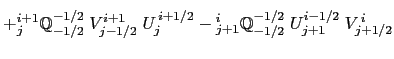
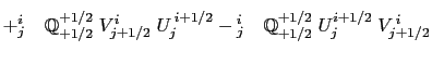
The summation is done over all
| ||||
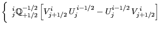 |
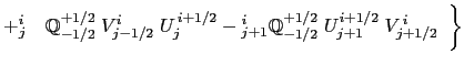
![$\displaystyle \biggl\{ {^{i}_j}\mathbb{Q}^{-1/2}_{+1/2} \left[ V^{i}_{j+1/2} U^{ i-1/2}_{j} - U^{i-1/2}_{j} V^{ i}_{j+1/2} \right]$](img1542.png) |
|||
![$\displaystyle + {^{i}_j}\mathbb{Q}^{-1/2}_{-1/2} \left[ V^{i}_{j-1/2} U^{ i-1/2}_{j} - U^{i-1/2}_{j} V^{ i}_{j-1/2} \right] \biggr.$](img1543.png) |
||||
![$\displaystyle + {^{i}_j}\mathbb{Q}^{+1/2}_{+1/2} \left[ V^{i}_{j+1/2} U^{ i+1/2}_{j} - U^{i+1/2}_{j} V^{ i}_{j+1/2} \right] \biggr.$](img1544.png) |
||||
![$\displaystyle + {^{i}_j}\mathbb{Q}^{+1/2}_{-1/2} \left[ V^{i}_{j-1/2} U^{ i...
...j} - U^{i+1/2}_{j-1} V^{ i}_{j-1/2} \right] \; \biggr\} \qquad \equiv 0$](img1545.png) |
||||
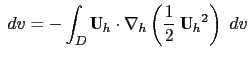
The change of Kinetic Energy (KE) due to the vertical advection is exactly balanced by the change of KE due to the horizontal gradient of KE :
 and operator)
applied in the horizontal and vertical directions, it becomes:
and operator)
applied in the horizontal and vertical directions, it becomes:
 KEG KEG |
|||||
 |
|||||
|
|||||
|
 |
||||
|
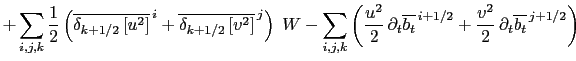
Assuming that  and and
| |||||
|
|||||
|
|||||
|
|||||
|
The first term provides the discrete expression for the vertical advection of momentum (ZAD), while the second term corresponds exactly to (C.7), therefore:
| |||||
 ZAD ZAD |
|||||
There is two main points here. First, the satisfaction of this property links the choice of
the discrete formulation of the vertical advection and of the horizontal gradient
of KE. Choosing one imposes the other. For example KE can also be discretized
as
 . This leads to the following
expression for the vertical advection:
. This leads to the following
expression for the vertical advection:
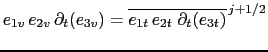
Second, as soon as the chosen ![]() -coordinate depends on time, an extra constraint
arises on the time derivative of the volume at
-coordinate depends on time, an extra constraint
arises on the time derivative of the volume at ![]() - and
- and  -points:
 |
|
 |
 |
(C.10) |
| (C.11) |
Blah blah required on the the step representation of bottom topography.....
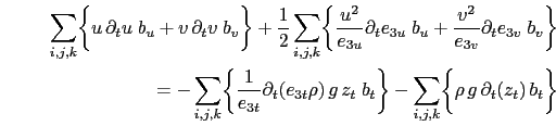
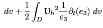
When the equation of state is linear (![]() when an advection-diffusion equation
for density can be derived from those of temperature and salinity) the change of
KE due to the work of pressure forces is balanced by the change of potential
energy due to buoyancy forces:
when an advection-diffusion equation
for density can be derived from those of temperature and salinity) the change of
KE due to the work of pressure forces is balanced by the change of potential
energy due to buoyancy forces:
This property can be satisfied in a discrete sense for both ![]() - and
- and ![]() -coordinates.
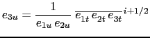
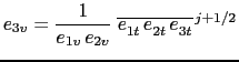
Indeed, defining the depth of a
-coordinates.
Indeed, defining the depth of a ![]() -point,
-point, ![]() , as the sum of the vertical scale
factors at
, as the sum of the vertical scale
factors at ![]() -points starting from the surface, the work of pressure forces can be
written as:
-points starting from the surface, the work of pressure forces can be
written as:
![$\displaystyle - \int_D \left. \nabla p \right\vert _z \cdot \textbf{U}_h \;dv \...
...1/2} [p_t] - g\;\overline \rho^{ i+1/2}\;\delta_{i+1/2} [z_t] \Bigr) \; u\;b_u$](img1573.png) |
||||
|
Using successively (4.11),
| ||||
 |
||||
|
||||
 is equal to the last term of (C.7).
In other words, the following property must be satisfied:
is equal to the last term of (C.7).
In other words, the following property must be satisfied:
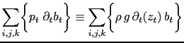
Let introduce ![]() the pressure at
the pressure at ![]() -point such that
-point such that
![$ \delta_k [p_w] = - \rho g e_{3t}$](img1587.png) .
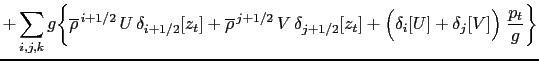
The right-hand-side of the above equation can be transformed as follows:
.
The right-hand-side of the above equation can be transformed as follows:
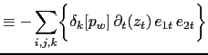 |
![$\displaystyle \equiv - \sum\limits_{i,j,k} \biggl\{ \delta_k [p_w] \partial_t (z_t) e_{1t} e_{2t} \biggr\}$](img1589.png) |
|
 |
||
 |
 |
Note that this property strongly constrains the discrete expression of both
the depth of ![]() points and of the term added to the pressure gradient in the
points and of the term added to the pressure gradient in the
![]() -coordinate. Nevertheless, it is almost never satisfied since a linear equation
of state is rarely used.
-coordinate. Nevertheless, it is almost never satisfied since a linear equation
of state is rarely used.
Gurvan Madec and the NEMO Team
NEMO European Consortium2017-02-17