Continuous conservation

The discretization of pimitive equation in $ s$-coordinate ($ i.e.$ time and space varying vertical coordinate) must be chosen so that the discrete equation of the model satisfy integral constrains on energy and enstrophy.

Let us first establish those constraint in the continuous world. The total energy ($ i.e.$ kinetic plus potential energies) is conserved :

$\displaystyle \partial_t \left( \int_D \left( \frac{1}{2} {\textbf{U}_h}^2 + \rho   g   z \right) \;dv \right) =$ 0 (C.3)

under the following assumptions: no dissipation, no forcing (wind, buoyancy flux, atmospheric pressure variations), mass conservation, and closed domain.

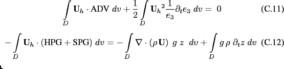
This equation can be transformed to obtain several sub-equalities. The transformation for the advection term depends on whether the vector invariant form or the flux form is used for the momentum equation. Using (C.2) and introducing (A.15) in (C.3) for the former form and Using (C.1) and introducing (A.16) in (C.3) for the latter form leads to:

$\displaystyle \par advection term (vector invariant form): \begin{equation}\int...
...ht)\;g\;z\;\;dv + \int\limits_D g  \rho \; \partial_t z \;dv  \end{equation}$ (C.4a)

where $ \nabla_h = \left. \nabla \right\vert _k$ is the gradient along the $ s$-surfaces.

blah blah.... $  $
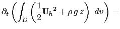
The prognostic ocean dynamics equation can be summarized as follows:

NXT$\displaystyle = \dbinom {\text{VOR} + \text{KEG} + \text {ZAD} } {\text{COR} + \text{ADV} } + \text{HPG} + \text{SPG} + \text{LDF} + \text{ZDF}$    

$  $

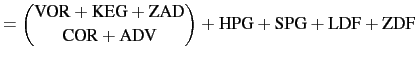
Vector invariant form:

$\displaystyle \begin{equation}\int\limits_D \textbf{U}_h \cdot \text{VOR} \;dv ...
...ht)\;g\;z\;\;dv + \int\limits_D g  \rho \; \partial_t z \;dv  \end{equation}$    

Flux form:

$\displaystyle \begin{equation}\int\limits_D \textbf{U}_h \cdot \text {COR} \; d...
...ht)\;g\;z\;\;dv + \int\limits_D g  \rho \; \partial_t z \;dv  \end{equation}$    

$  $

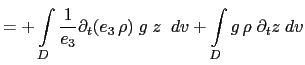
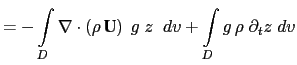
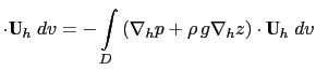
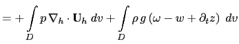
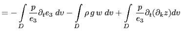
(C.6c) is the balance between the conversion KE to PE and PE to KE. Indeed the left hand side of (C.6c) can be transformed as follows:

$\displaystyle \partial_t \left( \int\limits_D { \rho   g   z \;dv} \right)$ $\displaystyle = + \int\limits_D \frac{1}{e_3} \partial_t (e_3 \rho) \;g\;z\;\;dv + \int\limits_D g  \rho \; \partial_t z \;dv$    
  $\displaystyle = - \int\limits_D \nabla \cdot \left( \rho  \textbf {U} \right)\;g\;z\;\;dv + \int\limits_D g  \rho \; \partial_t z \;dv$    
  $\displaystyle = + \int\limits_D \rho  g \left( \textbf {U}_h \cdot \nabla_h z ...
...1}{e_3} \partial_k z \right) \;dv + \int\limits_D g  \rho \; \partial_t z \;dv$    
  $\displaystyle = + \int\limits_D \rho  g \left( \omega + \partial_t z + \textbf {U}_h \cdot \nabla_h z \right) \;dv$    
  $\displaystyle =+ \int\limits_D g  \rho \; w \; dv$    

where the last equality is obtained by noting that the brackets is exactly the expression of $ w$, the vertical velocity referenced to the fixe $ z$-coordinate system (see (A.5)).

The left hand side of (C.6c) can be transformed as follows:

$\displaystyle - \int\limits_D \left. \nabla p \right\vert _z$ $\displaystyle \cdot \textbf{U}_h \;dv = - \int\limits_D \left( \nabla_h p + \rho   g \nabla_h z \right) \cdot \textbf{U}_h \;dv$    
$\displaystyle \allowdisplaybreaks$ $\displaystyle = - \int\limits_D \nabla_h p \cdot \textbf{U}_h \;dv - \int\limits_D \rho   g   \nabla_h z \cdot \textbf{U}_h \;dv$    
$\displaystyle \allowdisplaybreaks$ $\displaystyle = +\int\limits_D p  \nabla_h \cdot \textbf{U}_h \;dv + \int\limits_D \rho   g \left( \omega - w + \partial_t z \right) \;dv$    
$\displaystyle \allowdisplaybreaks$ $\displaystyle = -\int\limits_D p \left( \frac{1}{e_3} \partial_t e_3 + \frac{1}...
...ht) \;dv +\int\limits_D \rho   g \left( \omega - w + \partial_t z \right) \;dv$    
$\displaystyle \allowdisplaybreaks$ $\displaystyle = -\int\limits_D \frac{p}{e_3} \partial_t e_3 \;dv +\int\limits_D...
...ega \;dv +\int\limits_D \rho   g \left( \omega - w + \partial_t z \right) \;dv$    
  $\displaystyle = -\int\limits_D \frac{p}{e_3} \partial_t e_3 \;dv -\int\limits_D...
...ega \;dv +\int\limits_D \rho   g \left( \omega - w + \partial_t z \right) \;dv$    
  $\displaystyle = - \int\limits_D \frac{p}{e_3} \partial_t e_3 \; \;dv - \int\limits_D \rho   g   w \;dv + \int\limits_D \rho   g   \partial_t z \;dv$    

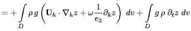
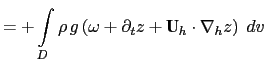
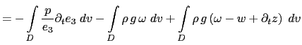
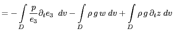
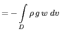
introducing the hydrostatic balance $ \partial_k p=-\rho  g e_3$ in the last term, it becomes:


$\displaystyle \allowdisplaybreaks$ $\displaystyle = - \int\limits_D \frac{p}{e_3} \partial_t e_3 \;dv - \int\limits...
...o   g   w \;dv - \int\limits_D \frac{1}{e_3} \partial_k p  \partial_t z \;dv$    
  $\displaystyle = - \int\limits_D \frac{p}{e_3} \partial_t e_3 \;dv - \int\limits...
...ho   g   w \;dv + \int\limits_D  \frac{p}{e_3}\partial_t ( \partial_k z ) dv$    
  $\displaystyle = - \int\limits_D \rho   g   w \;dv$    

Gurvan Madec and the NEMO Team
NEMO European Consortium2017-02-17