Next: Continuous conservation Up: Discrete Invariants of the Previous: Discrete Invariants of the Contents Index
Notation used in this appendix in the demonstations :
fluxes at the faces of a ![]() -box:
-box:
volume of cells at ![]() -,
-,  -, and
 ![]() -points:
-points:
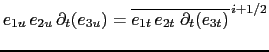
partial derivative notation:
![]()
![]() is the volume element, with only
is the volume element, with only ![]() that depends on time.
that depends on time.
![]() and
and ![]() are the ocean domain volume and surface, respectively.
No wetting/drying is allow (
are the ocean domain volume and surface, respectively.
No wetting/drying is allow (![]()
![]() )
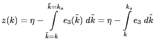
Let
)
Let ![]() and
and ![]() be the ocean surface and bottom, resp.
(
be the ocean surface and bottom, resp.
(![]()
![]() and
and ![]() , where
, where ![]() is the bottom depth).
is the bottom depth).
 |
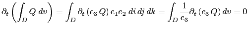
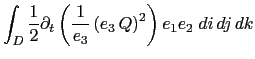
Continuity equation with the above notation:
![$\displaystyle \frac{1}{e_{3t}} \partial_t (e_{3t})+ \frac{1}{b_t} \biggl\{ \delta_i [U] + \delta_j [V] + \delta_k [W] \biggr\} = 0$](img1484.png) |
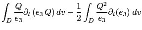
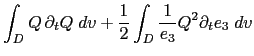
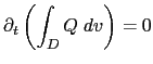
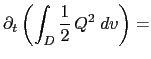
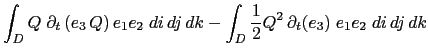
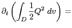
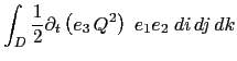
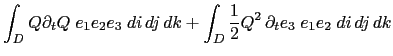
A quantity, ![]() is conserved when its domain averaged time change is zero, that is when:
is conserved when its domain averaged time change is zero, that is when:
 |
 |
 |
 |
|
 |
 |
 |
|
 |
Gurvan Madec and the NEMO Team
NEMO European Consortium2017-02-17