Diagnosing the Steric effect in sea surface height

Changes in steric sea level are caused when changes in the density of the water column imply an expansion or contraction of the column. It is essentially produced through surface heating/cooling and to a lesser extent through non-linear effects of the equation of state (cabbeling, thermobaricity...). Non-Boussinesq models contain all ocean effects within the ocean acting on the sea level. In particular, they include the steric effect. In contrast, Boussinesq models, such as NEMO, conserve volume, rather than mass, and so do not properly represent expansion or contraction. The steric effect is therefore not explicitely represented. This approximation does not represent a serious error with respect to the flow field calculated by the model [Greatbatch, 1994], but extra attention is required when investigating sea level, as steric changes are an important contribution to local changes in sea level on seasonal and climatic time scales. This is especially true for investigation into sea level rise due to global warming.

Fortunately, the steric contribution to the sea level consists of a spatially uniform component that can be diagnosed by considering the mass budget of the world ocean [Greatbatch, 1994]. In order to better understand how global mean sea level evolves and thus how the steric sea level can be diagnosed, we compare, in the following, the non-Boussinesq and Boussinesq cases.

Let denote $\mathcal{M}$ the total mass of liquid seawater ( $\mathcal{M}=\int_D \rho dv$), $\mathcal{V}$ the total volume of seawater ( $\mathcal{V}=\int_D dv$), $\mathcal{A}$ the total surface of the ocean ( $\mathcal{A}=\int_S ds$), $\bar{\rho}$ the global mean seawater (in situ) density ( $\bar{\rho}= 1/\mathcal{V} \int_D \rho dv$), and $\bar{\eta}$ the global mean sea level ( $\bar{\eta}=1/\mathcal{A}\int_S \eta ds$).

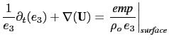
A non-Boussinesq fluid conserves mass. It satisfies the following relations:

$$\begin{split}\mathcal{M} &= \mathcal{V} \;\bar{\rho} \mathcal{V} &= \mathcal{A} \;\bar{\eta} \end{split}$$ (11.3)

Temporal changes in total mass is obtained from the density conservation equation :

$$\frac{1}{e_3} \partial_t ( e_3 \rho) + \nabla( \rho \textbf{U} ) = \left. \frac{\textit{emp}}{e_3}\right\vert _\textit{surface}$$ (11.4)

where $\rho$ is the in situ density, and emp the surface mass exchanges with the other media of the Earth system (atmosphere, sea-ice, land). Its global averaged leads to the total mass change

$$\partial_t \mathcal{M} = \mathcal{A} \;\overline{\textit{emp}}$$ (11.5)

where $\overline{\textit{emp}}=\int_S \textit{emp} ds$ is the net mass flux through the ocean surface. Bringing (11.5) and the time derivative of (11.3) together leads to the evolution equation of the mean sea level

$$\partial_t \bar{\eta} = \frac{\overline{\textit{emp}}}{ \bar{\rho}} - \frac{\mathcal{V}}{\mathcal{A}} \;\frac{\partial_t \bar{\rho} }{\bar{\rho}}$$ (11.6)

The first term in equation (11.6) alters sea level by adding or subtracting mass from the ocean. The second term arises from temporal changes in the global mean density; $i.e.$ from steric effects.

In a Boussinesq fluid, $\rho$ is replaced by $\rho_o$ in all the equation except when $\rho$ appears multiplied by the gravity ($i.e.$ in the hydrostatic balance of the primitive Equations). In particular, the mass conservation equation, (11.4), degenerates into the incompressibility equation:

$$\frac{1}{e_3} \partial_t ( e_3 ) + \nabla( \textbf{U} ) = \left. \frac{\textit{emp}}{\rho_o e_3}\right\vert _ \textit{surface}$$ (11.7)

and the global average of this equation now gives the temporal change of the total volume,

$$\partial_t \mathcal{V} = \mathcal{A} \;\frac{\overline{\textit{emp}}}{\rho_o}$$ (11.8)

Only the volume is conserved, not mass, or, more precisely, the mass which is conserved is the Boussinesq mass, $\mathcal{M}_o = \rho_o \mathcal{V}$. The total volume (or equivalently the global mean sea level) is altered only by net volume fluxes across the ocean surface, not by changes in mean mass of the ocean: the steric effect is missing in a Boussinesq fluid.

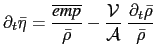
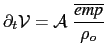
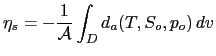
Nevertheless, following [Greatbatch, 1994], the steric effect on the volume can be diagnosed by considering the mass budget of the ocean. The apparent changes in $\mathcal{M}$, mass of the ocean, which are not induced by surface mass flux must be compensated by a spatially uniform change in the mean sea level due to expansion/contraction of the ocean [Greatbatch, 1994]. In others words, the Boussinesq mass, $\mathcal{M}_o$, can be related to $\mathcal{M}$, the total mass of the ocean seen by the Boussinesq model, via the steric contribution to the sea level, $\eta_s$, a spatially uniform variable, as follows:

$$\mathcal{M}_o = \mathcal{M} + \rho_o \eta_s \mathcal{A}$$ (11.9)

Any change in $\mathcal{M}$ which cannot be explained by the net mass flux through the ocean surface is converted into a mean change in sea level. Introducing the total density anomaly, $\mathcal{D}= \int_D d_a dv$, where $d_a= (\rho -\rho_o ) / \rho_o$ is the density anomaly used in NEMO (cf. §5.8.1) in (11.9) leads to a very simple form for the steric height:

$$\eta_s = - \frac{1}{\mathcal{A}} \mathcal{D}$$ (11.10)

The above formulation of the steric height of a Boussinesq ocean requires four remarks. First, one can be tempted to define $\rho_o$ as the initial value of $\mathcal{M}/\mathcal{V}$, $i.e.$ set $\mathcal{D}_{t=0}=0$, so that the initial steric height is zero. We do not recommend that. Indeed, in this case $\rho_o$ depends on the initial state of the ocean. Since $\rho_o$ has a direct effect on the dynamics of the ocean (it appears in the pressure gradient term of the momentum equation) it is definitively not a good idea when inter-comparing experiments. We better recommend to fixe once for all $\rho_o$ to $1035\;Kg m^{-3}$. This value is a sensible choice for the reference density used in a Boussinesq ocean climate model since, with the exception of only a small percentage of the ocean, density in the World Ocean varies by no more than 2$\%$ from this value (Gill [1982], page 47).

Second, we have assumed here that the total ocean surface, $\mathcal{A}$, does not change when the sea level is changing as it is the case in all global ocean GCMs (wetting and drying of grid point is not allowed).

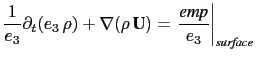
Third, the discretisation of (11.10) depends on the type of free surface which is considered. In the non linear free surface case, $i.e.$ key_ vvl defined, it is given by

$$\eta_s = - \frac{ \sum_{i, j, k} d_a\; e_{1t} e_{2t} e_{3t} } { \sum_{i, j, k} e_{1t} e_{2t} e_{3t} }$$ (11.11)

whereas in the linear free surface, the volume above the z=0 surface must be explicitly taken into account to better approximate the total ocean mass and thus the steric sea level:

$$\eta_s = - \frac{ \sum_{i, j, k} d_a\; e_{1t}e_{2t}e_{3t} + \su... ... \eta } {\sum_{i, j, k} e_{1t}e_{2t}e_{3t} + \sum_{i, j} e_{1t}e_{2t} \eta }$$ (11.12)

The fourth and last remark concerns the effective sea level and the presence of sea-ice. In the real ocean, sea ice (and snow above it) depresses the liquid seawater through its mass loading. This depression is a result of the mass of sea ice/snow system acting on the liquid ocean. There is, however, no dynamical effect associated with these depressions in the liquid ocean sea level, so that there are no associated ocean currents. Hence, the dynamically relevant sea level is the effective sea level, $i.e.$ the sea level as if sea ice (and snow) were converted to liquid seawater [Campin et al., 2008]. However, in the current version of NEMO the sea-ice is levitating above the ocean without mass exchanges between ice and ocean. Therefore the model effective sea level is always given by $\eta + \eta_s$, whether or not there is sea ice present.

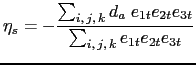
In AR5 outputs, the thermosteric sea level is demanded. It is steric sea level due to changes in ocean density arising just from changes in temperature. It is given by:

$$\eta_s = - \frac{1}{\mathcal{A}} \int_D d_a(T,S_o,p_o) dv$$ (11.13)

where $S_o$ and $p_o$ are the initial salinity and pressure, respectively.

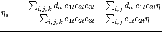
Both steric and thermosteric sea level are computed in diaar5.F90 which needs the key_ diaar5 defined to be called.