Miscellaneous options

Diurnal cycle (sbcdcy.F90)

Figure 7.2: Example of recontruction of the diurnal cycle variation of short wave flux from daily mean values. The reconstructed diurnal cycle (black line) is chosen as the mean value of the analytical cycle (blue line) over a time step, not as the mid time step value of the analytically cycle (red square). From Bernie et al. [2007].

Bernie et al. [2005] have shown that to capture 90$\%$ of the diurnal variability of SST requires a vertical resolution in upper ocean of 1 m or better and a temporal resolution of the surface fluxes of 3 h or less. Unfortunately high frequency forcing fields are rare, not to say inexistent. Nevertheless, it is possible to obtain a reasonable diurnal cycle of the SST knowning only short wave flux (SWF) at high frequency [Bernie et al., 2007]. Furthermore, only the knowledge of daily mean value of SWF is needed, as higher frequency variations can be reconstructed from them, assuming that the diurnal cycle of SWF is a scaling of the top of the atmosphere diurnal cycle of incident SWF. The Bernie et al. [2007] reconstruction algorithm is available in NEMO by setting ln_dm2dc = true (a namsbc namelist variable) when using CORE bulk formulea (ln_blk_core = true) or the flux formulation (ln_flx = true). The reconstruction is performed in the sbcdcy.F90 module. The detail of the algoritm used can be found in the appendix A of Bernie et al. [2007]. The algorithm preserve the daily mean incomming SWF as the reconstructed SWF at a given time step is the mean value of the analytical cycle over this time step (Fig.7.2). The use of diurnal cycle reconstruction requires the input SWF to be daily ($i.e.$ a frequency of 24 and a time interpolation set to true in sn_qsr namelist parameter). Furthermore, it is recommended to have a least 8 surface module time step per day, that is $\rdt \textit{nn\_fsbc}\index{Namelist variables!nn\_fsbc} < 10,800 s = 3 h$. An example of recontructed SWF is given in Fig.7.3 for a 12 reconstructed diurnal cycle, one every 2 hours (from 1am to 11pm).

Figure 7.3: Example of recontruction of the diurnal cycle variation of short wave flux from daily mean values on an ORCA2 grid with a time sampling of 2 hours (from 1am to 11pm). The display is on (i,j) plane.

Note also that the setting a diurnal cycle in SWF is highly recommended when the top layer thickness approach 1 m or less, otherwise large error in SST can appear due to an inconsistency between the scale of the vertical resolution and the forcing acting on that scale.

Rotation of vector pairs onto the model grid directions

When using a flux (ln_flx=true) or bulk (ln_clio=true or ln_core=true) formulation, pairs of vector components can be rotated from east-north directions onto the local grid directions. This is particularly useful when interpolation on the fly is used since here any vectors are likely to be defined relative to a rectilinear grid. To activate this option a non-empty string is supplied in the rotation pair column of the relevant namelist. The eastward component must start with "U" and the northward component with "V". The remaining characters in the strings are used to identify which pair of components go together. So for example, strings "U1" and "V1" next to "utau" and "vtau" would pair the wind stress components together and rotate them on to the model grid directions; "U2" and "V2" could be used against a second pair of components, and so on. The extra characters used in the strings are arbitrary. The rot_rep routine from the geo2ocean.F90 module is used to perform the rotation.

Surface restoring to observed SST and/or SSS (sbcssr.F90)

!-----------------------------------------------------------------------
&namsbc_ssr    !   surface boundary condition : sea surface restoring
!-----------------------------------------------------------------------
!              !  file name  ! frequency (hours) ! variable  ! time interp. !  clim  ! 'yearly'/ ! weights  ! rotation ! land/sea mask !
!              !             !  (if <0  months)  !   name    !   (logical)  !  (T/F) ! 'monthly' ! filename ! pairing  ! filename      !
   sn_sst      = 'sst_data'  ,        24         ,  'sst'    ,    .false.   , .false., 'yearly'  , ''       , ''       , ''
   sn_sss      = 'sss_data'  ,        -1         ,  'sss'    ,    .true.    , .true. , 'yearly'  , ''       , ''       , ''

   cn_dir      = './'      !  root directory for the location of the runoff files
   nn_sstr     =     0     !  add a retroaction term in the surface heat       flux (=1) or not (=0)
   nn_sssr     =     2     !  add a damping     term in the surface freshwater flux (=2)
                           !  or to SSS only (=1) or no damping term (=0)
   rn_dqdt     =   -40.    !  magnitude of the retroaction on temperature   [W/m2/K]
   rn_deds     =  -166.67  !  magnitude of the damping on salinity   [mm/day]
   ln_sssr_bnd =   .true.  !  flag to bound erp term (associated with nn_sssr=2)
   rn_sssr_bnd =   4.e0    !  ABS(Max/Min) value of the damping erp term [mm/day]
/

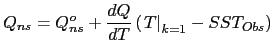
IOptions are defined through the namsbc_ssr namelist variables. n forced mode using a flux formulation (ln_flx = true), a feedback term must be added to the surface heat flux $Q_{ns}^o$:

$$Q_{ns} = Q_{ns}^o + \frac{dQ}{dT} \left( \left. T \right\vert _{k=1} - SST_{Obs} \right)$$ (7.8)

where SST is a sea surface temperature field (observed or climatological), $T$ is the model surface layer temperature and $\frac{dQ}{dT}$ is a negative feedback coefficient usually taken equal to $-40 W/m^2/K$. For a $50 m$ mixed-layer depth, this value corresponds to a relaxation time scale of two months. This term ensures that if $T$ perfectly matches the supplied SST, then $Q$ is equal to $Q_o$.

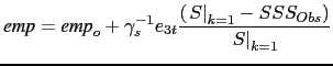
In the fresh water budget, a feedback term can also be added. Converted into an equivalent freshwater flux, it takes the following expression :

$$\textit{emp} = \textit{emp}_o + \gamma_s^{-1} e_{3t} \frac{ \left(\left.S\right\vert _{k=1}-SSS_{Obs}\right)} {\left.S\right\vert _{k=1}}$$ (7.9)

where $\textit{emp}_{o }$ is a net surface fresh water flux (observed, climatological or an atmospheric model product), SSS$_{Obs}$ is a sea surface salinity (usually a time interpolation of the monthly mean Polar Hydrographic Climatology [Steele et al., 2001]), $\left.S\right\vert _{k=1}$ is the model surface layer salinity and $\gamma_s$ is a negative feedback coefficient which is provided as a namelist parameter. Unlike heat flux, there is no physical justification for the feedback term in 7.9 as the atmosphere does not care about ocean surface salinity [Madec and Delecluse, 1997]. The SSS restoring term should be viewed as a flux correction on freshwater fluxes to reduce the uncertainties we have on the observed freshwater budget.

Handling of ice-covered area (sbcice_...)

The presence at the sea surface of an ice covered area modifies all the fluxes transmitted to the ocean. There are several way to handle sea-ice in the system depending on the value of the nn_ice namelist parameter found in namsbc namelist.

nn_ice = 0

there will never be sea-ice in the computational domain. This is a typical namelist value used for tropical ocean domain. The surface fluxes are simply specified for an ice-free ocean. No specific things is done for sea-ice.

nn_ice = 1

sea-ice can exist in the computational domain, but no sea-ice model is used. An observed ice covered area is read in a file. Below this area, the SST is restored to the freezing point and the heat fluxes are set to $-4 W/m^2$ ($-2 W/m^2$) in the northern (southern) hemisphere. The associated modification of the freshwater fluxes are done in such a way that the change in buoyancy fluxes remains zero. This prevents deep convection to occur when trying to reach the freezing point (and so ice covered area condition) while the SSS is too large. This manner of managing sea-ice area, just by using si IF case, is usually referred as the ice-if model. It can be found in the sbcice_if.F90 module.

nn_ice = 2 or more

A full sea ice model is used. This model computes the ice-ocean fluxes, that are combined with the air-sea fluxes using the ice fraction of each model cell to provide the surface ocean fluxes. Note that the activation of a sea-ice model is is done by defining a CPP key (key_ lim2, key_ lim3 or key_ cice). The activation automatically overwrites the read value of nn_ice to its appropriate value ($i.e.$ $2$ for LIM-2, $3$ for LIM-3 or $4$ for CICE).

Interface to CICE (sbcice_cice.F90)

It is now possible to couple a regional or global NEMO configuration (without AGRIF) to the CICE sea-ice model by using key_ cice. The CICE code can be obtained from LANL and the additional 'hadgem3' drivers will be required, even with the latest code release. Input grid files consistent with those used in NEMO will also be needed, and CICE CPP keys ORCA_GRID, CICE_IN_NEMO and coupled should be used (seek advice from UKMO if necessary). Currently the code is only designed to work when using the CORE forcing option for NEMO (with calc_strair = true and calc_Tsfc = true in the CICE name-list), or alternatively when NEMO is coupled to the HadGAM3 atmosphere model (with calc_strair = false and calc_Tsfc = false). The code is intended to be used with nn_fsbc set to 1 (although coupling ocean and ice less frequently should work, it is possible the calculation of some of the ocean-ice fluxes needs to be modified slightly - the user should check that results are not significantly different to the standard case).

There are two options for the technical coupling between NEMO and CICE. The standard version allows complete flexibility for the domain decompositions in the individual models, but this is at the expense of global gather and scatter operations in the coupling which become very expensive on larger numbers of processors. The alternative option (using key_ nemocice_decomp for both NEMO and CICE) ensures that the domain decomposition is identical in both models (provided domain parameters are set appropriately, and processor_shape = square-ice and distribution_wght = block in the CICE name-list) and allows much more efficient direct coupling on individual processors. This solution scales much better although it is at the expense of having more idle CICE processors in areas where there is no sea ice.

Freshwater budget control (sbcfwb.F90)

For global ocean simulation it can be useful to introduce a control of the mean sea level in order to prevent unrealistic drift of the sea surface height due to inaccuracy in the freshwater fluxes. In NEMO, two way of controlling the the freshwater budget.

nn_fwb=0

no control at all. The mean sea level is free to drift, and will certainly do so.

nn_fwb=1

global mean emp set to zero at each model time step.

nn_fwb=2

freshwater budget is adjusted from the previous year annual mean budget which is read in the EMPave_old.dat file. As the model uses the Boussinesq approximation, the annual mean fresh water budget is simply evaluated from the change in the mean sea level at January the first and saved in the EMPav.dat file.

Neutral drag coefficient from external wave model (sbcwave.F90)

!-----------------------------------------------------------------------
&namsbc_wave   ! External fields from wave model
!-----------------------------------------------------------------------
!              !  file name  ! frequency (hours) ! variable     ! time interp. !  clim   ! 'yearly'/ ! weights  ! rotation ! land/sea mask !
!              !             !  (if <0  months)  !   name       !   (logical)  !  (T/F)  ! 'monthly' ! filename ! pairing  ! filename      !
   sn_cdg      =  'cdg_wave' ,        1          , 'drag_coeff' ,     .true.   , .false. , 'daily'   ,  ''      , ''       , ''
   sn_usd      =  'sdw_wave' ,        1          , 'u_sd2d'     ,     .true.   , .false. , 'daily'   ,  ''      , ''       , ''
   sn_vsd      =  'sdw_wave' ,        1          , 'v_sd2d'     ,     .true.   , .false. , 'daily'   ,  ''      , ''       , ''
   sn_wn       =  'sdw_wave' ,        1          , 'wave_num'   ,     .true.   , .false. , 'daily'   ,  ''      , ''       , ''
!
   cn_dir_cdg  = './'  !  root directory for the location of drag coefficient files
/

In order to read a neutral drag coeff, from an external data source ($i.e.$ a wave model), the logical variable ln_cdgw in namsbc namelist must be set to true. The sbcwave.F90 module containing the routine sbc_wave reads the namelist namsbc_wave (for external data names, locations, frequency, interpolation and all the miscellanous options allowed by Input Data generic Interface see §7.2) and a 2D field of neutral drag coefficient. Then using the routine TURB_CORE_1Z or TURB_CORE_2Z, and starting from the neutral drag coefficent provided, the drag coefficient is computed according to stable/unstable conditions of the air-sea interface following Large and Yeager [2004].