Input Data generic interface

A generic interface has been introduced to manage the way input data (2D or 3D fields, like surface forcing or ocean T and S) are specify in NEMO. This task is archieved by fldread.F90. The module was design with four main objectives in mind:

1. optionally provide a time interpolation of the input data at model time-step, whatever their input frequency is, and according to the different calendars available in the model.
2. optionally provide an on-the-fly space interpolation from the native input data grid to the model grid.
3. make the run duration independent from the period cover by the input files.
4. provide a simple user interface and a rather simple developer interface by limiting the number of prerequisite information.

As a results the user have only to fill in for each variable a structure in the namelist file to defined the input data file and variable names, the frequency of the data (in hours or months), whether its is climatological data or not, the period covered by the input file (one year, month, week or day), and three additional parameters for on-the-fly interpolation. When adding a new input variable, the developer has to add the associated structure in the namelist, read this information by mirroring the namelist read in sbc_blk_init for example, and simply call fld_read to obtain the desired input field at the model time-step and grid points.

The only constraints are that the input file is a NetCDF file, the file name follows a nomenclature (see §7.2.1), the period it cover is one year, month, week or day, and, if on-the-fly interpolation is used, a file of weights must be supplied (see §7.2.2).

Note that when an input data is archived on a disc which is accessible directly from the workspace where the code is executed, then the use can set the cn_dir to the pathway leading to the data. By default, the data are assumed to have been copied so that cn_dir='./'.

Input Data specification (fldread.F90)

The structure associated with an input variable contains the following information:

      

!  file name  ! frequency (hours) ! variable  ! time interp. !  clim  ! 'yearly'/ ! weights  ! rotation ! land/sea mask ! 

!             !  (if <0  months)  !   name    !   (logical)  !  (T/F) ! 'monthly' ! filename ! pairing  ! filename      !

where

File name

: the stem name of the NetCDF file to be open. This stem will be completed automatically by the model, with the addition of a '.nc' at its end and by date information and possibly a prefix (when using AGRIF). Tab.7.2 provides the resulting file name in all possible cases according to whether it is a climatological file or not, and to the open/close frequency (see below for definition).

Table 7.2: naming nomenclature for climatological or interannual input file, as a function of the Open/close frequency. The stem name is assumed to be 'fn'. For weekly files, the 'LLL' corresponds to the first three letters of the first day of the week ($i.e.$ 'sun','sat','fri','thu','wed','tue','mon'). The 'YYYY', 'MM' and 'DD' should be replaced by the actual year/month/day, always coded with 4 or 2 digits. Note that (1) in mpp, if the file is split over each subdomain, the suffix '.nc' is replaced by '_PPPP.nc', where 'PPPP' is the process number coded with 4 digits; (2) when using AGRIF, the prefix '_N' is added to files, where 'N' is the child grid number.

	daily or weekLLL	monthly	yearly
clim = false	fn_yYYYYmMMdDD	fn_yYYYYmMM	fn_yYYYY
clim = true	not possible	fn_m??.nc	fn

Record frequency

: the frequency of the records contained in the input file. Its unit is in hours if it is positive (for example 24 for daily forcing) or in months if negative (for example -1 for monthly forcing or -12 for annual forcing). Note that this frequency must really be an integer and not a real. On some computers, seting it to '24.' can be interpreted as 240!

Variable name

: the name of the variable to be read in the input NetCDF file.

Time interpolation

: a logical to activate, or not, the time interpolation. If set to 'false', the forcing will have a steplike shape remaining constant during each forcing period. For example, when using a daily forcing without time interpolation, the forcing remaining constant from 00h00'00” to 23h59'59". If set to 'true', the forcing will have a broken line shape. Records are assumed to be dated the middle of the forcing period. For example, when using a daily forcing with time interpolation, linear interpolation will be performed between mid-day of two consecutive days.

Climatological forcing

: a logical to specify if a input file contains climatological forcing which can be cycle in time, or an interannual forcing which will requires additional files if the period covered by the simulation exceed the one of the file. See the above the file naming strategy which impacts the expected name of the file to be opened.

Open/close frequency

: the frequency at which forcing files must be opened/closed. Four cases are coded: 'daily', 'weekLLL' (with 'LLL' the first 3 letters of the first day of the week), 'monthly' and 'yearly' which means the forcing files will contain data for one day, one week, one month or one year. Files are assumed to contain data from the beginning of the open/close period. For example, the first record of a yearly file containing daily data is Jan 1st even if the experiment is not starting at the beginning of the year.

Others

: 'weights filename', 'pairing rotation' and 'land/sea mask' are associted with on-the-fly interpolation which is described in §7.2.2.

Additional remarks:
(1) The time interpolation is a simple linear interpolation between two consecutive records of the input data. The only tricky point is therefore to specify the date at which we need to do the interpolation and the date of the records read in the input files. Following Leclair and Madec [2009], the date of a time step is set at the middle of the time step. For example, for an experiment starting at 0h00'00" with a one hour time-step, a time interpolation will be performed at the following time: 0h30'00", 1h30'00", 2h30'00", etc. However, for forcing data related to the surface module, values are not needed at every time-step but at every nn_fsbc time-step. For example with nn_fsbc = 3, the surface module will be called at time-steps 1, 4, 7, etc. The date used for the time interpolation is thus redefined to be at the middle of nn_fsbc time-step period. In the previous example, this leads to: 1h30'00", 4h30'00", 7h30'00", etc.
(2) For code readablility and maintenance issues, we don't take into account the NetCDF input file calendar. The calendar associated with the forcing field is build according to the information provided by user in the record frequency, the open/close frequency and the type of temporal interpolation. For example, the first record of a yearly file containing daily data that will be interpolated in time is assumed to be start Jan 1st at 12h00'00" and end Dec 31st at 12h00'00".
(3) If a time interpolation is requested, the code will pick up the needed data in the previous (next) file when interpolating data with the first (last) record of the open/close period. For example, if the input file specifications are ”yearly, containing daily data to be interpolated in time”, the values given by the code between 00h00'00" and 11h59'59" on Jan 1st will be interpolated values between Dec 31st 12h00'00" and Jan 1st 12h00'00". If the forcing is climatological, Dec and Jan will be keep-up from the same year. However, if the forcing is not climatological, at the end of the open/close period the code will automatically close the current file and open the next one. Note that, if the experiment is starting (ending) at the beginning (end) of an open/close period we do accept that the previous (next) file is not existing. In this case, the time interpolation will be performed between two identical values. For example, when starting an experiment on Jan 1st of year Y with yearly files and daily data to be interpolated, we do accept that the file related to year Y-1 is not existing. The value of Jan 1st will be used as the missing one for Dec 31st of year Y-1. If the file of year Y-1 exists, the code will read its last record. Therefore, this file can contain only one record corresponding to Dec 31st, a useful feature for user considering that it is too heavy to manipulate the complete file for year Y-1.

Interpolation on-the-Fly

Interpolation on the Fly allows the user to supply input files required for the surface forcing on grids other than the model grid. To do this he or she must supply, in addition to the source data file, a file of weights to be used to interpolate from the data grid to the model grid. The original development of this code used the SCRIP package (freely available here under a copyright agreement). In principle, any package can be used to generate the weights, but the variables in the input weights file must have the same names and meanings as assumed by the model. Two methods are currently available: bilinear and bicubic interpolation. Prior to the interpolation, providing a land/sea mask file, the user can decide to remove land points from the input file and substitute the corresponding values with the average of the 8 neighbouring points in the native external grid. Only "sea points" are considered for the averaging. The land/sea mask file must be provided in the structure associated with the input variable. The netcdf land/sea mask variable name must be 'LSM' it must have the same horizontal and vertical dimensions of the associated variable and should be equal to 1 over land and 0 elsewhere. The procedure can be recursively applied setting nn_lsm > 1 in namsbc namelist. Note that nn_lsm=0 forces the code to not apply the procedure even if a file for land/sea mask is supplied.

Bilinear Interpolation

The input weights file in this case has two sets of variables: src01, src02, src03, src04 and wgt01, wgt02, wgt03, wgt04. The "src" variables correspond to the point in the input grid to which the weight "wgt" is to be applied. Each src value is an integer corresponding to the index of a point in the input grid when written as a one dimensional array. For example, for an input grid of size 5x10, point (3,2) is referenced as point 8, since (2-1)*5+3=8. There are four of each variable because bilinear interpolation uses the four points defining the grid box containing the point to be interpolated. All of these arrays are on the model grid, so that values src01(i,j) and wgt01(i,j) are used to generate a value for point (i,j) in the model.

Symbolically, the algorithm used is:

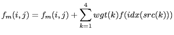$$f_{m}(i,j) = f_{m}(i,j) + \sum_{k=1}^{4} {wgt(k)f(idx(src(k)))}$$ (7.1)

where function idx() transforms a one dimensional index src(k) into a two dimensional index, and wgt(1) corresponds to variable "wgt01" for example.

Bicubic Interpolation

Again there are two sets of variables: "src" and "wgt". But in this case there are 16 of each. The symbolic algorithm used to calculate values on the model grid is now:

$$\begin{split}f_{m}(i,j) = f_{m}(i,j) +& \sum_{k=1}^{4} {wgt(k... ...{\partial i \partial j}\right\vert _{idx(src(k))} } \end{split}$$

The gradients here are taken with respect to the horizontal indices and not distances since the spatial dependency has been absorbed into the weights.

Implementation

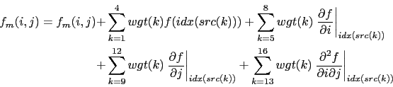To activate this option, a non-empty string should be supplied in the weights filename column of the relevant namelist; if this is left as an empty string no action is taken. In the model, weights files are read in and stored in a structured type (WGT) in the fldread module, as and when they are first required. This initialisation procedure determines whether the input data grid should be treated as cyclical or not by inspecting a global attribute stored in the weights input file. This attribute must be called "ew_wrap" and be of integer type. If it is negative, the input non-model grid is assumed not to be cyclic. If zero or greater, then the value represents the number of columns that overlap. $E.g.$ if the input grid has columns at longitudes 0, 1, 2, .... , 359, then ew_wrap should be set to 0; if longitudes are 0.5, 2.5, .... , 358.5, 360.5, 362.5, ew_wrap should be 2. If the model does not find attribute ew_wrap, then a value of -999 is assumed. In this case the fld_read routine defaults ew_wrap to value 0 and therefore the grid is assumed to be cyclic with no overlapping columns. (In fact this only matters when bicubic interpolation is required.) Note that no testing is done to check the validity in the model, since there is no way of knowing the name used for the longitude variable, so it is up to the user to make sure his or her data is correctly represented.

Next the routine reads in the weights. Bicubic interpolation is assumed if it finds a variable with name "src05", otherwise bilinear interpolation is used. The WGT structure includes dynamic arrays both for the storage of the weights (on the model grid), and when required, for reading in the variable to be interpolated (on the input data grid). The size of the input data array is determined by examining the values in the "src" arrays to find the minimum and maximum i and j values required. Since bicubic interpolation requires the calculation of gradients at each point on the grid, the corresponding arrays are dimensioned with a halo of width one grid point all the way around. When the array of points from the data file is adjacent to an edge of the data grid, the halo is either a copy of the row/column next to it (non-cyclical case), or is a copy of one from the first few columns on the opposite side of the grid (cyclical case).

Limitations

1. The case where input data grids are not logically rectangular has not been tested.
2. This code is not guaranteed to produce positive definite answers from positive definite inputs when a bicubic interpolation method is used.
3. The cyclic condition is only applied on left and right columns, and not to top and bottom rows.
4. The gradients across the ends of a cyclical grid assume that the grid spacing between the two columns involved are consistent with the weights used.
5. Neither interpolation scheme is conservative. (There is a conservative scheme available in SCRIP, but this has not been implemented.)

Utilities

A set of utilities to create a weights file for a rectilinear input grid is available (see the directory NEMOGCM/TOOLS/WEIGHTS).

Standalone Surface Boundary Condition Scheme

!-----------------------------------------------------------------------
&namsbc_sas    !   analytical surface boundary condition
!-----------------------------------------------------------------------
!              !  file name  ! frequency (hours) ! variable  ! time interp. !  clim  ! 'yearly'/ ! weights  ! rotation ! land/sea mask !
!              !             !  (if <0  months)  !   name    !   (logical)  !  (T/F) ! 'monthly' ! filename ! pairing  ! filename      !
   sn_usp      = 'sas_grid_U' ,    120           , 'vozocrtx' ,  .true.    , .true. ,   'yearly'  , ''       , ''             , ''
   sn_vsp      = 'sas_grid_V' ,    120           , 'vomecrty' ,  .true.    , .true. ,   'yearly'  , ''       , ''             , ''
   sn_tem      = 'sas_grid_T' ,    120           , 'sosstsst' ,  .true.    , .true. ,   'yearly'  , ''       , ''             , ''
   sn_sal      = 'sas_grid_T' ,    120           , 'sosaline' ,  .true.    , .true. ,   'yearly'  , ''       , ''             , ''
   sn_ssh      = 'sas_grid_T' ,    120           , 'sossheig' ,  .true.    , .true. ,   'yearly'  , ''       , ''             , ''
   sn_e3t      = 'sas_grid_T' ,    120           , 'e3t_m'    ,  .true.    , .true. ,   'yearly'  , ''       , ''             , ''
   sn_frq      = 'sas_grid_T' ,    120           , 'frq_m'    ,  .true.    , .true. ,   'yearly'  , ''       , ''             , ''

   ln_3d_uve   = .true.    !  specify whether we are supplying a 3D u,v and e3 field
   ln_read_frq = .false.    !  specify whether we must read frq or not
   cn_dir      = './'      !  root directory for the location of the bulk files are
/

In some circumstances it may be useful to avoid calculating the 3D temperature, salinity and velocity fields and simply read them in from a previous run or receive them from OASIS. For example:

• Multiple runs of the model are required in code development to see the effect of different algorithms in the bulk formulae.
• The effect of different parameter sets in the ice model is to be examined.
• Development of sea-ice algorithms or parameterizations.
• spinup of the iceberg floats
• ocean/sea-ice simulation with both media running in parallel (ln_mixcpl = true)

The StandAlone Surface scheme provides this utility. Its options are defined through the namsbc_sas namelist variables. A new copy of the model has to be compiled with a configuration based on ORCA2_SAS_LIM. However no namelist parameters need be changed from the settings of the previous run (except perhaps nn_date0) In this configuration, a few routines in the standard model are overriden by new versions. Routines replaced are:

• nemogcm.F90 : This routine initialises the rest of the model and repeatedly calls the stp time stepping routine (step.F90) Since the ocean state is not calculated all associated initialisations have been removed.
• step.F90 : The main time stepping routine now only needs to call the sbc routine (and a few utility functions).
• sbcmod.F90 : This has been cut down and now only calculates surface forcing and the ice model required. New surface modules that can function when only the surface level of the ocean state is defined can also be added (e.g. icebergs).
• daymod.F90 : No ocean restarts are read or written (though the ice model restarts are retained), so calls to restart functions have been removed. This also means that the calendar cannot be controlled by time in a restart file, so the user must make sure that nn_date0 in the model namelist is correct for his or her purposes.
• stpctl.F90 : Since there is no free surface solver, references to it have been removed from stp_ctl module.
• diawri.F90 : All 3D data have been removed from the output. The surface temperature, salinity and velocity components (which have been read in) are written along with relevant forcing and ice data.

One new routine has been added:

• sbcsas.F90 : This module initialises the input files needed for reading temperature, salinity and velocity arrays at the surface. These filenames are supplied in namelist namsbc_sas. Unfortunately because of limitations with the iom.F90 module, the full 3D fields from the mean files have to be read in and interpolated in time, before using just the top level. Since fldread is used to read in the data, Interpolation on the Fly may be used to change input data resolution.