Here (2.36)
is the  -component of the slope of the iso-neutral surface relative to the computational
surface, and
-component of the slope of the iso-neutral surface relative to the computational
surface, and  is the
  -component.
We will find it useful to consider the fluxes per unit area in 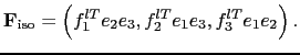 space; we write
 |
(D.2) |
Additionally, we will sometimes write the contributions towards the
fluxes  and
and
 from the component
 of
of  as
as  ,
,
 , with
 (no summation) etc.
The off-diagonal terms of the small angle diffusion tensor
(2.35), (D.1c) produce skew-fluxes along the
- and -directions resulting from the vertical tracer gradient:
The vertical diffusive flux associated with the  component of the small angle diffusion tensor is
 |
(D.5) |
Since there are no cross terms involving  and in the above, we can
consider the iso-neutral diffusive fluxes separately in the -
and in the above, we can
consider the iso-neutral diffusive fluxes separately in the - and -
planes, just adding together the vertical components from each
plane. The following description will describe the fluxes on the -
plane.
and -
planes, just adding together the vertical components from each
plane. The following description will describe the fluxes on the -
plane.
There is no natural discretization for the -component of the
skew-flux, (D.3), as
although it must be evaluated at  -points, it involves vertical
gradients (both for the tracer and the slope ), defined at
-points, it involves vertical
gradients (both for the tracer and the slope ), defined at
 -points. Similarly, the vertical skew flux, (D.4), is evaluated at
-points but involves horizontal gradients defined at -points.
-points. Similarly, the vertical skew flux, (D.4), is evaluated at
-points but involves horizontal gradients defined at -points.
The straightforward approach to discretize the lateral skew flux
(D.3) from tracer cell  to
to  , introduced in 1995
into OPA, (5.9), is to calculate a mean vertical
gradient at the -point from the average of the four surrounding
vertical tracer gradients, and multiply this by a mean slope at the
-point, calculated from the averaged surrounding vertical density
gradients. The total area-integrated skew-flux (flux per unit area in
, introduced in 1995
into OPA, (5.9), is to calculate a mean vertical
gradient at the -point from the average of the four surrounding
vertical tracer gradients, and multiply this by a mean slope at the
-point, calculated from the averaged surrounding vertical density
gradients. The total area-integrated skew-flux (flux per unit area in
 space) from tracer cell
to , noting that the
space) from tracer cell
to , noting that the
 in the area
 at the -point cancels out with
the
at the -point cancels out with
the
 associated with the vertical tracer
gradient, is then (5.9)
associated with the vertical tracer
gradient, is then (5.9)
where
and here and in the following we drop the  superscript from
 for simplicity.
Unfortunately the resulting combination
for simplicity.
Unfortunately the resulting combination
 of a average and a difference reduces to
 , so two-grid-point oscillations are
invisible to this discretization of the iso-neutral operator. These
computational modes will not be damped by this operator, and
may even possibly be amplified by it. Consequently, applying this
operator to a tracer does not guarantee the decrease of its
global-average variance. To correct this, we introduced a smoothing of
the slopes of the iso-neutral surfaces (see §9). This
technique works for
, so two-grid-point oscillations are
invisible to this discretization of the iso-neutral operator. These
computational modes will not be damped by this operator, and
may even possibly be amplified by it. Consequently, applying this
operator to a tracer does not guarantee the decrease of its
global-average variance. To correct this, we introduced a smoothing of
the slopes of the iso-neutral surfaces (see §9). This
technique works for  and
and  in so far as they are active tracers
(
in so far as they are active tracers
( they enter the computation of density), but it does not work
for a passive tracer.
[Griffies et al., 1998] introduce a different discretization of the
off-diagonal terms that nicely solves the problem.
they enter the computation of density), but it does not work
for a passive tracer.
[Griffies et al., 1998] introduce a different discretization of the
off-diagonal terms that nicely solves the problem.
Figure D.1:
(a) Arrangement of triads  and tracer gradients to
give lateral tracer flux from box to
(b) Triads
and tracer gradients to
give lateral tracer flux from box to
(b) Triads  and tracer gradients to give vertical tracer flux from
box to
and tracer gradients to give vertical tracer flux from
box to  .
.
|
|
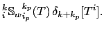
They get the skew flux from the products of the vertical gradients at
each -point surrounding the -point with the corresponding `triad'
slope calculated from the lateral density gradient across the -point
divided by the vertical density gradient at the same -point as the
tracer gradient. See Fig. D.1a, where the thick lines
denote the tracer gradients, and the thin lines the corresponding
triads, with slopes
 . The total area-integrated
skew-flux from tracer cell to
. The total area-integrated
skew-flux from tracer cell to
where the contributions of the triad fluxes are weighted by areas
 , and
, and  is now defined at the tracer points
rather than the -points. This discretization gives a much closer
stencil, and disallows the two-point computational modes.
is now defined at the tracer points
rather than the -points. This discretization gives a much closer
stencil, and disallows the two-point computational modes.
The vertical skew flux (D.4) from tracer cell to at the
-point
 is constructed similarly (Fig. D.1b)
by multiplying lateral tracer gradients from each of the four
surrounding -points by the appropriate triad slope:
is constructed similarly (Fig. D.1b)
by multiplying lateral tracer gradients from each of the four
surrounding -points by the appropriate triad slope:
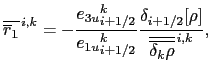
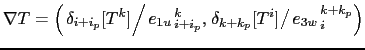
We notate the triad slopes  and
and  in terms of the `anchor point'
(appearing in both the vertical and lateral gradient), and the - and
-points
in terms of the `anchor point'
(appearing in both the vertical and lateral gradient), and the - and
-points  ,
,  at the centres of the `arms' of the
triad as follows (see also Fig. D.1):
at the centres of the `arms' of the
triad as follows (see also Fig. D.1):
![$\displaystyle _i^k \mathbb{R}_{i_p}^{k_p} =-\frac{ {e_{3w}}_{ i}^{ k+k_p}} { ...
...eft(\alpha / \beta \right)_i^k \delta_{k+k_p}[T^i ] - \delta_{k+k_p}[S^i ] }.$](img1766.png) |
(D.6) |
In calculating the slopes of the local neutral
surfaces, the expansion coefficients  and
and  are
evaluated at the anchor points of the triad D.3, while the metrics are
calculated at the - and -points on the arms.
are
evaluated at the anchor points of the triad D.3, while the metrics are
calculated at the - and -points on the arms.
Figure D.2:
Triad notation for quarter cells. -cells are inside
boxes, while the  -cell is shaded in green and the
 -cell is shaded in pink.
|
|
Each triad
 is associated (Fig. D.2) with the quarter
cell that is the intersection of the -cell, the
is associated (Fig. D.2) with the quarter
cell that is the intersection of the -cell, the  -cell and the
  -cell. Expressing the slopes and
in (D.6) and (D.7) in this notation, we have
e.g.
-cell. Expressing the slopes and
in (D.6) and (D.7) in this notation, we have
e.g.
 . Each triad slope
 is used once (as an
  ) to calculate the
lateral flux along its -arm, at , and then again as an
) to calculate the
lateral flux along its -arm, at , and then again as an
 to calculate the vertical flux along its -arm at
. Each vertical area
to calculate the vertical flux along its -arm at
. Each vertical area  used to calculate the lateral
flux and horizontal area
used to calculate the lateral
flux and horizontal area  used to calculate the vertical flux
can also be identified as the area across the - and -arms of a
unique triad, and we notate these areas, similarly to the triad
slopes, as
used to calculate the vertical flux
can also be identified as the area across the - and -arms of a
unique triad, and we notate these areas, similarly to the triad
slopes, as
 ,
,
 , where e.g. in (D.6)
 , and in (D.7)
 .
.
A key property of iso-neutral diffusion is that it should not affect
the (locally referenced) density. In particular there should be no
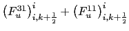
lateral or vertical density flux. The lateral density flux disappears so long as the
area-integrated lateral diffusive flux from tracer cell to
coming from the  term of the diffusion tensor takes the
form
term of the diffusion tensor takes the
form
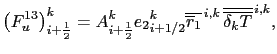
![$\displaystyle \left( F_u^{11} \right) _{i+\frac{1}{2}} ^{k} = - \left( \Alts_i^...
...{4} \right) \frac{\delta _{i+1/2} \left[ T^k\right]}{{e_{1u}}_{ i+1/2}^{ k}},$](img1783.png) |
(D.7) |
where the areas are as in (D.6). In this case,
separating the total lateral flux, the sum of (D.6) and
(D.9), into triad components, a lateral tracer
flux
![$\displaystyle _i^k {\mathbb{F}_u}_{i_p}^{k_p} (T) = - \Alts_i^k{ \:}_i^k{\mathb...
...{i_p}^{k_p}} \frac{ \delta_{k+k_p} [T^i] }{{e_{3w}}_{ i}^{ k+k_p} } \right)$](img1784.png) |
(D.8) |
can be identified with each triad. Then, because the
same metric factors
 and
and
 are employed for both the density gradients
in
and the tracer gradients, the lateral
density flux associated with each triad separately disappears.
are employed for both the density gradients
in
and the tracer gradients, the lateral
density flux associated with each triad separately disappears.
 |
(D.9) |
Thus the total flux
 from tracer cell
to must also vanish since it is a sum of four such triad fluxes.
from tracer cell
to must also vanish since it is a sum of four such triad fluxes.
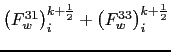
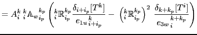
The squared slope  in the expression (D.5) for the
component is also expressed in terms of area-weighted
squared triad slopes, so the area-integrated vertical flux from tracer
cell to resulting from the term is
in the expression (D.5) for the
component is also expressed in terms of area-weighted
squared triad slopes, so the area-integrated vertical flux from tracer
cell to resulting from the term is
![$\displaystyle \left( F_w^{33} \right) _i^{k+\frac{1}{2}} = - \left( \Alts_i^{k+...
...\Alts_i^k a_{4}' s_{4}'^2 \right)\delta_{k+\frac{1}{2}} \left[ T^{i+1} \right],$](img1790.png) |
(D.10) |
where the areas  and slopes are the same as in
(D.7).
Then, separating the total vertical flux, the sum of (D.7) and
(D.12), into triad components, a vertical flux
and slopes are the same as in
(D.7).
Then, separating the total vertical flux, the sum of (D.7) and
(D.12), into triad components, a vertical flux
may be associated with each triad. Each vertical density flux
 associated with a triad then separately disappears (because the
lateral flux
associated with a triad then separately disappears (because the
lateral flux
 disappears). Consequently the total vertical density flux
 from tracer cell
to must also vanish since it is a sum of four such triad
fluxes.
from tracer cell
to must also vanish since it is a sum of four such triad
fluxes.
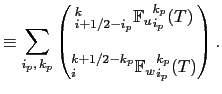
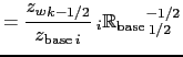
We can explicitly identify (Fig. D.2) the triads associated with the , , and , used in the definition of
the -fluxes and -fluxes in
(D.7), (D.6), (D.9) (D.12) and
Fig. D.1 to write out the iso-neutral fluxes at - and
-points as sums of the triad fluxes that cross the - and -faces:
Ensuring the scheme does not increase tracer variance
We now require that this operator should not increase the
globally-integrated tracer variance.
Each triad slope
drives a lateral flux
 across the -point and
a vertical flux
across the -point and
a vertical flux
 across the
-point . The lateral flux drives a net rate of change of
variance, summed over the two -points
across the
-point . The lateral flux drives a net rate of change of
variance, summed over the two -points
 and
and
 , of
, of
while the vertical flux similarly drives a net rate of change of
variance summed over the -points
 (above) and
 (below) of
![$\displaystyle _i^k{\mathbb{F}_w}_{i_p}^{k_p} (T) \delta_{k+ k_p}[T^i].$](img1807.png) |
(D.14) |
The total variance tendency driven by the triad is the sum of these
two. Expanding
and
with (D.10) and
(D.13), it is
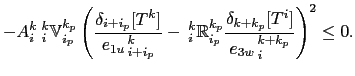
The key point is then that if we require
and
to be related to a triad volume
 by
by
 |
(D.15) |
the variance tendency reduces to the perfect square
![$\displaystyle -\Alts_i^k{\:} _i^k\mathbb{V}_{i_p}^{k_p} \left( \frac{ \delta_{i...
...{k_p} \frac{ \delta_{k+k_p} [T^i] }{{e_{3w}}_{ i}^{ k+k_p} } \right)^2\leq 0.$](img1811.png) |
(D.16) |
Thus, the constraint (D.18) ensures that the fluxes (D.10, D.13) associated
with a given slope triad
do not increase
the net variance. Since the total fluxes are sums of such fluxes from
the various triads, this constraint, applied to all triads, is
sufficient to ensure that the globally integrated variance does not
increase.
The expression (D.18) can be interpreted as a discretization
of the global integral
 |
(D.17) |
where, within each triad volume
, the
lateral and vertical fluxes/unit area
and the gradient
To complete the discretization we now need only specify the triad
volumes
. Griffies et al. [1998] identify
these
as the volumes of the quarter
cells, defined in terms of the distances between , , and
-points. This is the natural discretization of
(D.20). The NEMO model, however, operates with scale
factors instead of grid sizes, and scale factors for the quarter
cells are not defined. Instead, therefore we simply choose
and
-points. This is the natural discretization of
(D.20). The NEMO model, however, operates with scale
factors instead of grid sizes, and scale factors for the quarter
cells are not defined. Instead, therefore we simply choose
 |
(D.18) |
as a quarter of the volume of the -cell inside which the triad
quarter-cell lies. This has the nice property that when the slopes
 vanish, the lateral flux from tracer cell to
reduces to the classical form
vanish, the lateral flux from tracer cell to
reduces to the classical form
![$\displaystyle -\overline\Alts_{ i+1/2}^k\; \frac{{b_u}_{i+1/2}^k}{{e_{1u}}_{ ...
...:{e_{1v}}_{ i + 1/2}^{ k}\;\delta_{i+ 1/2}[T^k]}{{e_{1u}}_{ i + 1/2}^{ k}}.$](img1817.png) |
(D.19) |
In fact if the diffusive coefficient is defined at -points, so that
we employ
 instead of
  in the definitions of the
triad fluxes (D.10) and (D.13),
we can replace
in the definitions of the
triad fluxes (D.10) and (D.13),
we can replace
 by
by
 in the above.
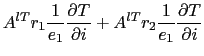
The iso-neutral fluxes at - and
-points are the sums of the triad fluxes that cross the - and
-faces (D.15):
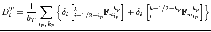
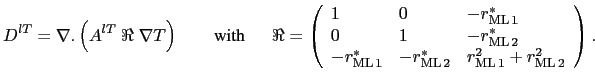
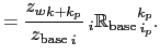
Thus the diffusion operator within the mixed layer is given by:
![$\displaystyle D^{lT}=\nabla {\rm {\bf .}}\left( {A^{lT}\;\Re \;\nabla T} \right...
...hfill & {-\rML[2]} \hfill & {\rML[1]^2+\rML[2]^2} \hfill \end{array} }} \right)$](img1843.png) |
(D.30) |
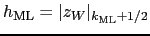
This slope tapering gives a natural connection between tracer in the
mixed-layer and in isopycnal layers immediately below, in the
thermocline. It is consistent with the way the
 are
tapered within the mixed layer (see §D.3.5 below)
so as to ensure a uniform GM eddy-induced velocity throughout the
mixed layer. However, it gives a downwards density flux and so acts so
as to reduce potential energy in the same way as does the slope
limiting discussed above in §D.2.9.
are
tapered within the mixed layer (see §D.3.5 below)
so as to ensure a uniform GM eddy-induced velocity throughout the
mixed layer. However, it gives a downwards density flux and so acts so
as to reduce potential energy in the same way as does the slope
limiting discussed above in §D.2.9.
As in §D.2.9 above, the tapering
(D.32a) is applied separately to each triad
 , and the
adjusted. For clarity, we assume
, and the
adjusted. For clarity, we assume
 -coordinates in the following; the conversion from
to
-coordinates in the following; the conversion from
to
 and back to
follows exactly as described
above by (D.31).
and back to
follows exactly as described
above by (D.31).
- Mixed-layer depth is defined so as to avoid including regions of weak
vertical stratification in the slope definition.
At each
 (simplified to in
Fig. D.4), we define the mixed-layer by setting
the vertical index of the tracer point immediately below the mixed
layer,
(simplified to in
Fig. D.4), we define the mixed-layer by setting
the vertical index of the tracer point immediately below the mixed
layer,
 , as the maximum (shallowest tracer point)
such that the potential density
, as the maximum (shallowest tracer point)
such that the potential density
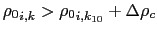 , where
  is
the tracer gridbox within which the depth reaches 10 m. See the left
side of Fig. D.4. We use the
is
the tracer gridbox within which the depth reaches 10 m. See the left
side of Fig. D.4. We use the  -gridbox
instead of the surface gridbox to avoid problems e.g. with thin
daytime mixed-layers. Currently we use the same
-gridbox
instead of the surface gridbox to avoid problems e.g. with thin
daytime mixed-layers. Currently we use the same
 for ML triad tapering as is
used to output the diagnosed mixed-layer depth
for ML triad tapering as is
used to output the diagnosed mixed-layer depth
 , the depth of the -point
above the
, the depth of the -point
above the
 tracer point.
- We define `basal' triad slopes
 as the slopes
of those triads whose vertical `arms' go down from the
tracer point to the
as the slopes
of those triads whose vertical `arms' go down from the
tracer point to the
 tracer point
below. This is to ensure that the vertical density gradients
associated with these basal triad slopes
are
representative of the thermocline. The four basal triads defined in the bottom part
of Fig. D.4 are then
tracer point
below. This is to ensure that the vertical density gradients
associated with these basal triad slopes
are
representative of the thermocline. The four basal triads defined in the bottom part
of Fig. D.4 are then
The vertical flux associated with each of these triads passes through the -point
 lying below the
tracer point,
so it is this depth
lying below the
tracer point,
so it is this depth
 |
(D.32) |
(one gridbox deeper than the
diagnosed ML depth
 that sets the
  used to taper
the slopes in (D.32a).
used to taper
the slopes in (D.32a).
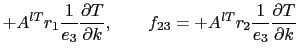
- Finally, we calculate the adjusted triads
 within the mixed
layer, by multiplying the appropriate
by the ratio of
the depth of the -point
within the mixed
layer, by multiplying the appropriate
by the ratio of
the depth of the -point
 to
to
 . For
instance the green triad centred on
. For
instance the green triad centred on
Figure D.4:
Definition of
mixed-layer depth and calculation of linearly tapered
triads. The figure shows a water column at a given
(simplified to ), with the ocean surface at the top. Tracer points are denoted by
bullets, and black lines the edges of the tracer cells;
increases upwards.
We define the mixed-layer by setting the vertical index
of the tracer point immediately below the mixed layer,
, as the maximum (shallowest tracer point)
such that
,
where is the tracer gridbox within which the depth
reaches 10 m. We calculate the triad slopes within the mixed
layer by linearly tapering them from zero (at the surface) to
the `basal' slopes, the slopes of the four triads passing through the
-point
(blue square),
. Triads with
different  , denoted by different colours, (e.g. the green
triad
, denoted by different colours, (e.g. the green
triad
 ) are tapered to the appropriate basal triad.
![\includegraphics[width=0.60\textwidth]{Fig_GRIFF_MLB_triads}](img1865.png) |
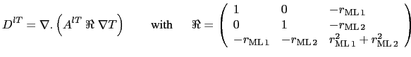
Additional truncation of skew iso-neutral flux
components
The alternative option is activated by setting ln_triad_iso =
true. This retains the same tapered slope 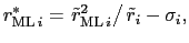 described above for the
calculation of the term of the iso-neutral diffusion tensor (the
vertical tracer flux driven by vertical tracer gradients), but
replaces the in the skew term by
described above for the
calculation of the term of the iso-neutral diffusion tensor (the
vertical tracer flux driven by vertical tracer gradients), but
replaces the in the skew term by
 |
(D.34) |
giving a ML diffusive operator
![$\displaystyle D^{lT}=\nabla {\rm {\bf .}}\left( {A^{lT}\;\Re \;\nabla T} \right...
...& {-\rML[2]^*} \hfill & {\rML[1]^2+\rML[2]^2} \hfill \end{array} }} \right).$](img1868.png) |
(D.35) |
This operator
D.4then has the property it gives no vertical density flux, and so does
not change the potential energy.
This approach is similar to multiplying the iso-neutral diffusion
coefficient by
 for steep
slopes, as suggested by Gerdes et al. [1991] (see also Griffies [2004]).
Again it is applied separately to each triad
for steep
slopes, as suggested by Gerdes et al. [1991] (see also Griffies [2004]).
Again it is applied separately to each triad
In practice, this approach gives weak vertical tracer fluxes through
the mixed-layer, as well as vanishing density fluxes. While it is
theoretically advantageous that it does not change the potential
energy, it may give a discontinuity between the
fluxes within the mixed-layer (purely horizontal) and just below (along
iso-neutral surfaces).
Footnotes
- ... triadD.3
- Note that in (D.8) we use the ratio
 instead of multiplying the temperature derivative by and the
salinity derivative by . This is more efficient as the ratio
can to be evaluated directly
instead of multiplying the temperature derivative by and the
salinity derivative by . This is more efficient as the ratio
can to be evaluated directly
- ... operatorD.4
- To ensure good behaviour where horizontal density
gradients are weak, we in fact follow Gerdes et al. [1991] and set
 .
.
Gurvan Madec and the NEMO Team
NEMO European Consortium2017-02-17
![$ \delta[S]$](img1833.png) in (D.16)
and (D.17). This results in a term similar to
(D.19),
in (D.16)
and (D.17). This results in a term similar to
(D.19),
![$\displaystyle = \Alts_i^k{\: }_i^k{\mathbb{A}_w}_{i_p}^{k_p} \left( {_i^k\mathb...
...p}}\right)^2 \frac{ \delta_{k+k_p} [T^i] }{{e_{3w}}_{ i}^{ k+k_p} } \right)$](img1793.png)