Next: Offline observation operator Up: Observation and model comparison Previous: Technical details Contents Index
Consider an observation point ![]() with
with longitude and latitude
with
with longitude and latitude
![]() and the
four nearest neighbouring model grid points
and the
four nearest neighbouring model grid points ![]() ,
, ![]() ,
, ![]() and
and ![]() with longitude and latitude (
with longitude and latitude (
![]() ,
,
![]() ),
(
),
(
![]() ,
,
![]() ) etc.
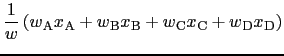
All horizontal interpolation methods implemented in NEMO
estimate the value of a model variable
) etc.
All horizontal interpolation methods implemented in NEMO
estimate the value of a model variable ![]() at point
at point ![]() as
a weighted linear combination of the values of the model
variables at the grid points
as
a weighted linear combination of the values of the model
variables at the grid points ![]() ,
, ![]() etc.:
etc.:
 |
(12.1) |
Four different possibilities are available for computing the weights.
| (12.2) |
 |
 |
(12.3) |
For many grids used by the NEMO model, such as the ORCA family,
the horizontal grid coordinates ![]() and
and ![]() are not simple functions
of latitude and longitude. Therefore, it is not always straightforward
to determine the grid points surrounding any given observational position.
Before the interpolation can be performed, a search
algorithm is then required to determine the corner points of
the quadrilateral cell in which the observation is located.
This is the most difficult and time consuming part of the
2D interpolation procedure.
A robust test for determining if an observation falls
within a given quadrilateral cell is as follows. Let
are not simple functions
of latitude and longitude. Therefore, it is not always straightforward
to determine the grid points surrounding any given observational position.
Before the interpolation can be performed, a search
algorithm is then required to determine the corner points of
the quadrilateral cell in which the observation is located.
This is the most difficult and time consuming part of the
2D interpolation procedure.
A robust test for determining if an observation falls
within a given quadrilateral cell is as follows. Let
![]() denote the observation point,
and let
denote the observation point,
and let
![]() ,
,
![]() ,
,
![]() and
and
![]() denote
the bottom left, bottom right, top left and top right
corner points of the cell, respectively.
To determine if P is inside
the cell, we verify that the cross-products
denote
the bottom left, bottom right, top left and top right
corner points of the cell, respectively.
To determine if P is inside
the cell, we verify that the cross-products
In order to speed up the grid search, there is the possibility to construct
a lookup table for a user specified resolution. This lookup
table contains the lower and upper bounds on the ![]() and
and ![]() indices
to be searched for on a regular grid. For each observation position,
the closest point on the regular grid of this position is computed and
the
indices
to be searched for on a regular grid. For each observation position,
the closest point on the regular grid of this position is computed and
the ![]() and
and ![]() ranges of this point searched to determine the precise
four points surrounding the observation.
ranges of this point searched to determine the precise
four points surrounding the observation.
For horizontal interpolation, there is the basic problem that the observations are unevenly distributed on the globe. In numerical models, it is common to divide the model grid into subgrids (or domains) where each subgrid is executed on a single processing element with explicit message passing for exchange of information along the domain boundaries when running on a massively parallel processor (MPP) system. This approach is used by NEMO.
For observations there is no natural distribution since the observations are not equally distributed on the globe. Two options have been made available: 1) geographical distribution; and 2) round-robin.
|
|
This is the simplest option in which the observations are distributed according
to the domain of the grid-point parallelization. Figure 12.1
shows an example of the distribution of the in situ data on processors
with a different colour for each observation
on a given processor for a 4 ![]() 2 decomposition with ORCA2.
The grid-point domain decomposition is clearly visible on the plot.
2 decomposition with ORCA2.
The grid-point domain decomposition is clearly visible on the plot.
The advantage of this approach is that all
information needed for horizontal interpolation is available without
any MPP communication. Of course, this is under the assumption that
we are only using a
![]() grid-point stencil for the interpolation
(e.g., bilinear interpolation). For higher order interpolation schemes this
is no longer valid. A disadvantage with the above scheme is that the number of
observations on each processor can be very different. If the cost of
the actual interpolation is expensive relative to the communication of
data needed for interpolation, this could lead to load imbalance.
grid-point stencil for the interpolation
(e.g., bilinear interpolation). For higher order interpolation schemes this
is no longer valid. A disadvantage with the above scheme is that the number of
observations on each processor can be very different. If the cost of
the actual interpolation is expensive relative to the communication of
data needed for interpolation, this could lead to load imbalance.
|
|
An alternative approach is to distribute the observations equally
among processors and use message passing in order to retrieve
the stencil for interpolation. The simplest distribution of the observations
is to distribute them using a round-robin scheme. Figure 12.2
shows the distribution of the in situ data on processors for the
round-robin distribution of observations with a different colour for
each observation on a given processor for a 4 ![]() 2 decomposition
with ORCA2 for the same input data as in Fig. 12.1.
The observations are now clearly randomly distributed on the globe.
In order to be able to perform horizontal interpolation in this case,
a subroutine has been developed that retrieves any grid points in the
global space.
2 decomposition
with ORCA2 for the same input data as in Fig. 12.1.
The observations are now clearly randomly distributed on the globe.
In order to be able to perform horizontal interpolation in this case,
a subroutine has been developed that retrieves any grid points in the
global space.
Vertical interpolation is achieved using either a cubic spline or linear interpolation. For the cubic spline, the top and bottom boundary conditions for the second derivative of the interpolating polynomial in the spline are set to zero. At the bottom boundary, this is done using the land-ocean mask.
Gurvan Madec and the NEMO Team
NEMO European Consortium2017-02-17
![\begin{displaymath}\begin{array}{lllll}
{{\bf r}_{}}_{\rm PA} \times {{\bf r}_{}...
...\; - \; {\phi_{}}_{\rm P} )] \; \widehat{\bf k} \\
\end{array}\end{displaymath}](img1276.png)