The Modified Leapfrog - Asselin Filter scheme
Significant changes have been introduced by Leclair and Madec [2009] in the
LF-RA scheme in order to ensure tracer conservation and to allow the use of
a much smaller value of the Asselin filter parameter. The modifications affect
both the forcing and filtering treatments in the LF-RA scheme.
In a classical LF-RA environment, the forcing term is centred in time,  it is time-stepped over a
  period:
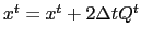 where
where  is the forcing applied to
  , and the time filter is given by (3.2)
so that is redistributed over several time step.
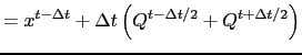
In the modified LF-RA environment, these two formulations have been replaced by:
, and the time filter is given by (3.2)
so that is redistributed over several time step.
In the modified LF-RA environment, these two formulations have been replaced by:
The change in the forcing formulation given by (3.9)
(see Fig.3.2) has a significant effect: the forcing term no
longer excites the divergence of odd and even time steps [Leclair and Madec, 2009].
This property improves the LF-RA scheme in two respects.
First, the LF-RA can now ensure the local and global conservation of tracers.
Indeed, time filtering is no longer required on the forcing part. The influence of
the Asselin filter on the forcing is be removed by adding a new term in the filter
(last term in (3.10) compared to (3.2)). Since
the filtering of the forcing was the source of non-conservation in the classical
LF-RA scheme, the modified formulation becomes conservative [Leclair and Madec, 2009].
Second, the LF-RA becomes a truly quasi-second order scheme. Indeed,
(3.9) used in combination with a careful treatment of static
instability (§10.2.2) and of the TKE physics (§10.1.4),
the two other main sources of time step divergence, allows a reduction by
two orders of magnitude of the Asselin filter parameter.
Note that the forcing is now provided at the middle of a time step:
 is the forcing applied over the
![$ [t,t+\rdt]$](img308.png) time interval. This and the change
in the time filter, (3.10), allows an exact evaluation of the
contribution due to the forcing term between any two time steps,
even if separated by only
time interval. This and the change
in the time filter, (3.10), allows an exact evaluation of the
contribution due to the forcing term between any two time steps,
even if separated by only  since the time filter is no longer applied to the
forcing term.
since the time filter is no longer applied to the
forcing term.
Figure:
Illustration of forcing integration methods.
(top) ”Traditional” formulation : the forcing is defined at the same time as the variable
to which it is applied (integer value of the time step index) and it is applied over a period.
(bottom) modified formulation : the forcing is defined in the middle of the time (integer and a half
value of the time step index) and the mean of two successive forcing values ( ,
,  ).
is applied over a period.
).
is applied over a period.
|
|
Gurvan Madec and the NEMO Team
NEMO European Consortium2017-02-17
![\includegraphics[width=0.90\textwidth]{Fig_MLF_forcing}](img309.png)
![$\displaystyle = x^t + \gamma \left[ x_F^{t-\rdt} - 2 x^t + x^{t+\rdt} \right] - \gamma \rdt \left[ Q^{t+\rdt/2} - Q^{t-\rdt/2} \right]$](img306.png)