Elliptic solvers (SOL)

!-----------------------------------------------------------------------
&namsol        !   elliptic solver / island / free surface
!-----------------------------------------------------------------------
   nn_solv     =      1    !  elliptic solver: =1 preconditioned conjugate gradient (pcg)
                           !                   =2 successive-over-relaxation (sor)
   nn_sol_arp  =      0    !  absolute/relative (0/1) precision convergence test
   rn_eps      =  1.e-6    !  absolute precision of the solver
   nn_nmin     =    300    !  minimum of iterations for the SOR solver
   nn_nmax     =    800    !  maximum of iterations for the SOR solver
   nn_nmod     =     10    !  frequency of test for the SOR solver
   rn_resmax   =  1.e-10   !  absolute precision for the SOR solver
   rn_sor      =  1.92     !  optimal coefficient for SOR solver (to be adjusted with the domain)
/

When the filtered sea surface height option is used, the surface pressure gradient is computed in dynspg_flt.F90. The force added in the momentum equation is solved implicitely. It is thus solution of an elliptic equation () for which two solvers are available: a Successive-Over-Relaxation scheme (SOR) and a preconditioned conjugate gradient scheme(PCG) [Madec, 1990, Madec et al., 1988]. The solver is selected trough the the value of nn_solv namsol namelist variable.

The PCG is a very efficient method for solving elliptic equations on vector computers. It is a fast and rather easy method to use; which are attractive features for a large number of ocean situations (variable bottom topography, complex coastal geometry, variable grid spacing, open or cyclic boundaries, etc ...). It does not require a search for an optimal parameter as in the SOR method. However, the SOR has been retained because it is a linear solver, which is a very useful property when using the adjoint model of NEMO.

At each time step, the time derivative of the sea surface height at time step $t+1$ (or equivalently the divergence of the after barotropic transport) that appears in the filtering forced is the solution of the elliptic equation obtained from the horizontal divergence of the vertical summation of (). Introducing the following coefficients:

$$\begin{aligned}&c_{i,j}^{NS} &&= {2 \rdt }^2 \; \frac{H_v (i,j)... ...u \right] - \delta_j \left[ e_{1v}M_v \right] , \end{aligned}$$

the resulting five-point finite difference equation is given by:

$$\begin{split}c_{i+1,j}^{NS} D_{i+1,j} + \; c_{i,j+1}^{EW} D_{... ...i,j}^{NS} + c_{i,j}^{EW} \right) D_{i,j} &= b_{i,j} \end{split}$$ (15.3)

(15.3) is a linear symmetric system of equations. All the elements of the corresponding matrix A vanish except those of five diagonals. With the natural ordering of the grid points (i.e. from west to east and from south to north), the structure of A is block-tridiagonal with tridiagonal or diagonal blocks. A is a positive-definite symmetric matrix of size $(jpi \cdot jpj)^2$, and B, the right hand side of (15.3), is a vector.

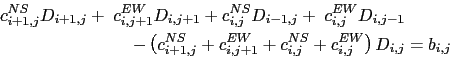
Note that in the linear free surface case, the depth that appears in (15.2) does not vary with time, and thus the matrix can be computed once for all. In non-linear free surface (key_ vvl defined) the matrix have to be updated at each time step.

Successive Over Relaxation (nn_solv=2, solsor.F90)

Let us introduce the four cardinal coefficients:

$$a_{i,j}^S = c_{i,j }^{NS}/d_{i,j} \qquad a_{i,j}^W = c_{i,j}^{EW}/d_{i,j}$$

$$a_{i,j}^E = c_{i,j+1}^{EW}/d_{i,j} \qquad a_{i,j}^N = c_{i+1,j}^{NS}/d_{i,j}$$

where $d_{i,j} = c_{i,j}^{NS}+ c_{i+1,j}^{NS} + c_{i,j}^{EW} + c_{i,j+1}^{EW}$ (i.e. the diagonal of the matrix). (15.3) can be rewritten as:

$$\begin{split}a_{i,j}^{N} D_{i+1,j} + a_{i,j}^{E} D_{i,j+1} +... ... a_{i,j}^{W} D_{i,j-1} - D_{i,j} = \tilde{b}_{i,j} \end{split}$$ (15.4)

with $\tilde b_{i,j} = b_{i,j}/d_{i,j}$. (15.4) is the equation actually solved with the SOR method. This method used is an iterative one. Its algorithm can be summarised as follows (see Haltiner and Williams [1980] for a further discussion):

initialisation (evaluate a first guess from previous time step computations)

$$D_{i,j}^0 = 2 D_{i,j}^t - D_{i,j}^{t-1}$$ (15.5)

iteration $n$, from $n=0$ until convergence, do :

$$\begin{split}R_{i,j}^n = &a_{i,j}^{N} D_{i+1,j}^n + a_{i,j}^... ...D_{i,j} ^{n+1} = &D_{i,j} ^{n} + \omega \;R_{i,j}^n \end{split}$$ (15.6)

where $\omega$ satisfies $1\leq \omega \leq 2$. An optimal value exists for $\omega$ which significantly accelerates the convergence, but it has to be adjusted empirically for each model domain (except for a uniform grid where an analytical expression for $\omega$ can be found [Richtmyer and Morton, 1967]). The value of $\omega$ is set using rn_sor, a namelist parameter. The convergence test is of the form:

$$\delta = \frac{\sum\limits_{i,j}{R_{i,j}^n}{R_{i,j}^n}} {\sum\limits_{i,j}{ \tilde{b}_{i,j}^n}{\tilde{b}_{i,j}^n}} \leq \epsilon$$ (15.7)

where $\epsilon$ is the absolute precision that is required. It is recommended that a value smaller or equal to $10^{-6}$ is used for $\epsilon$ since larger values may lead to numerically induced basin scale barotropic oscillations. The precision is specified by setting rn_eps (namelist parameter). In addition, two other tests are used to halt the iterative algorithm. They involve the number of iterations and the modulus of the right hand side. If the former exceeds a specified value, nn_max (namelist parameter), or the latter is greater than $10^{15}$, the whole model computation is stopped and the last computed time step fields are saved in a abort.nc NetCDF file. In both cases, this usually indicates that there is something wrong in the model configuration (an error in the mesh, the initial state, the input forcing, or the magnitude of the time step or of the mixing coefficients). A typical value of $nn\_max$ is a few hundred when $\epsilon = 10^{-6}$, increasing to a few thousand when $\epsilon = 10^{-12}$. The vectorization of the SOR algorithm is not straightforward. The scheme contains two linear recurrences on $i$ and $j$. This inhibits the vectorisation. (15.6) can be been rewritten as:

$$\begin{split}R_{i,j}^n = &a_{i,j}^{N} D_{i+1,j}^n + a_{i,j}^... ...n = &R_{i,j}^n - \omega \;a_{i,j}^{W}\; R_{i-1,j}^n \end{split}$$ (15.8)

This technique slightly increases the number of iteration required to reach the convergence, but this is largely compensated by the gain obtained by the suppression of the recurrences.

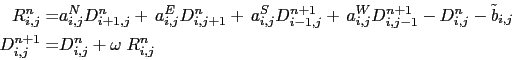
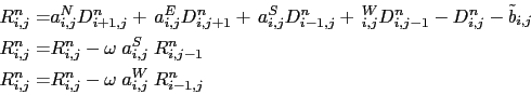
Another technique have been chosen, the so-called red-black SOR. It consist in solving successively (15.6) for odd and even grid points. It also slightly reduced the convergence rate but allows the vectorisation. In addition, and this is the reason why it has been chosen, it is able to handle the north fold boundary condition used in ORCA configuration ($i.e.$ tri-polar global ocean mesh).

The SOR method is very flexible and can be used under a wide range of conditions, including irregular boundaries, interior boundary points, etc. Proofs of convergence, etc. may be found in the standard numerical methods texts for partial differential equations.

Preconditioned Conjugate Gradient (nn_solv=1, solpcg.F90)

A is a definite positive symmetric matrix, thus solving the linear system (15.3) is equivalent to the minimisation of a quadratic functional:

$$\textbf{Ax} = \textbf{b} \leftrightarrow \textbf{x} = _{y} \phi (\textbf{y}) \quad , \qquad \phi (\textbf{y}) = 1/2 \langle \textbf{Ay},\textbf{y}\rangle - \langle \textbf{b},\textbf{y} \rangle$$

where $\langle , \rangle$ is the canonical dot product. The idea of the conjugate gradient method is to search for the solution in the following iterative way: assuming that $\textbf{x}^n$ has been obtained, $\textbf{x}^{n+1}$ is found from $\textbf {x}^{n+1}={\textbf {x}}^n+\alpha^n{\textbf {d}}^n$ which satisfies:

$${\textbf{ x}}^{n+1}= _{{\textbf{ y}}={\textbf{ x}}^n+\alpha^n {\textbf{ d}}^n} \phi ({\textbf{ y}})\;\;\Leftrightarrow \;\;\frac{d\phi }{d\alpha}=0$$

and expressing $\phi (\textbf{y})$ as a function of $\alpha$, we obtain the value that minimises the functional:

$$\alpha ^n = \langle{ \textbf{r}^n , \textbf{r}^n} \rangle / \langle {\textbf{ A d}^n, \textbf{d}^n} \rangle$$

where $\textbf{r}^n = \textbf{b}-\textbf{A x}^n = \textbf{A} (\textbf{x}-\textbf{x}^n)$ is the error at rank $n$. The descent vector $\textbf{d}^n$ s chosen to be dependent on the error: $\textbf{d}^n = \textbf{r}^n + \beta^n \textbf{d}^{n-1}$. $\beta ^n$ is searched such that the descent vectors form an orthogonal basis for the dot product linked to A. Expressing the condition $\langle \textbf{A d}^n, \textbf{d}^{n-1} \rangle = 0$ the value of $\beta ^n$ is found: $\beta ^n = \langle{ \textbf{r}^n , \textbf{r}^n} \rangle / \langle {\textbf{r}^{n-1}, \textbf{r}^{n-1}} \rangle$. As a result, the errors $\textbf{r}^n$ form an orthogonal base for the canonic dot product while the descent vectors $\textbf{d}^n$ form an orthogonal base for the dot product linked to A. The resulting algorithm is thus the following one:

initialisation :

$$\begin{split}\textbf{x}^0 &= D_{i,j}^0 = 2 D_{i,j}^t - D_{i,j... ..._0 &= \langle{ \textbf{r}^0 , \textbf{r}^0} \rangle \end{split}$$

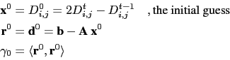iteration $n,$ from $n=0$ until convergence, do :

$$\begin{split}\text{z}^n& = \textbf{A d}^n \alpha_n &= \gam... ...= \textbf{r}^{n+1} + \beta_{n+1}\; \textbf{d}^{n} \end{split}$$ (15.9)

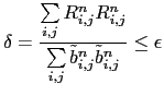
The convergence test is:

$$\delta = \gamma_{n}\; / \langle{ \textbf{b} , \textbf{b}} \rangle \leq \epsilon$$ (15.10)

where $\epsilon$ is the absolute precision that is required. As for the SOR algorithm, the whole model computation is stopped when the number of iterations, nn_max, or the modulus of the right hand side of the convergence equation exceeds a specified value (see §15.7.1 for a further discussion). The required precision and the maximum number of iterations allowed are specified by setting rn_eps and nn_max (namelist parameters).

It can be demonstrated that the above algorithm is optimal, provides the exact solution in a number of iterations equal to the size of the matrix, and that the convergence rate is faster as the matrix is closer to the identity matrix, $i.e.$ its eigenvalues are closer to 1. Therefore, it is more efficient to solve a better conditioned system which has the same solution. For that purpose, we introduce a preconditioning matrix Q which is an approximation of A but much easier to invert than A, and solve the system:

$$\textbf{Q}^{-1} \textbf{A x} = \textbf{Q}^{-1} \textbf{b}$$ (15.11)

The same algorithm can be used to solve (15.11) if instead of the canonical dot product the following one is used: ${\langle{ \textbf{a} , \textbf{b}} \rangle}_Q = \langle{ \textbf{a} , \textbf{Q b}} \rangle$, and if $\textbf{\ {b}} = \textbf{Q}^{-1}\;\textbf{b}$ and $\textbf{\ {A}} = \textbf{Q}^{-1}\;\textbf{A}$ are substituted to b and A [Madec et al., 1988]. In NEMO, Q is chosen as the diagonal of A, i.e. the simplest form for Q so that it can be easily inverted. In this case, the discrete formulation of (15.11) is in fact given by (15.4) and thus the matrix and right hand side are computed independently from the solver used.